1. Introduction

Machine learning (ML) studies how to learn patterns from data and apply them to unseen samples. Understanding it requires more than remembering model names: What signals does a model learn from, what assumptions guide its predictions, and how can we establish that it generalizes to real-world settings?

This article starts from the learning paradigm and modeling process, and introduces traditional machine learning, deep neural networks, pretrained models and generative models in sequence. Various methods are not simple substitution relationships: linear models are easy to explain and diagnose, tree models are suitable for many tabular tasks, and deep networks are good at learning complex representations; which one to choose requires a combination of data, evaluation indicators, and deployment costs.

Reading Guide

Intended readers: students, engineers and researchers who have basic programming, linear algebra and probability theory knowledge and want to establish a machine learning knowledge framework. This article focuses on the connection between classic principles and methods and does not serve as a ranking of the latest models.

reading objectives	Suggested Chapters	Questions to take away
Establish an overall understanding	§2 Basic Overview	What is the difference between learning signals, model assumptions, optimization and generalization?
Start a modeling project	§2.9 Experimental process	How to segment data, avoid leaks, and choose metrics?
Handle tabular and small-sample data	§3.2–§3.11 Traditional method	What are the prerequisites for linear models, tree models, and distance methods?
Understand deep learning	§3.12–§3.15 Deep Network	What are the differences in the structural preferences of MLP, CNN, RNN, and Transformer?
Understanding language models	§3.16 Pre-training and alignment	What problems do BERT, GPT, RLHF, and DPO solve respectively?
Understand generative and robot policies	§3.17–§3.20 generative models	How do GAN, VAE, diffusion and autoregression model distribution?
Choose a starting plan	§4 Selection and summary	How to establish a baseline and then determine whether a complex model is needed?

How to read this survey: Each section first gives the core points and intuition, and then introduces the mechanism, formulas and applicable boundaries. The suggestions in the table are experimental starting points and are not guarantees of algorithm performance. The robot direction can be combined with §2.2.3 reinforcement learning and §3.20.2 Diffusion Policy reading.

2. Basic overview of machine learning

2.1 What is machine learning?

Machine learning is a multi-field interdisciplinary subject involving probability theory, statistics, approximation theory, convex analysis, algorithm complexity theory, etc. Its core idea is: Let computers analyze data through algorithms, learn patterns from them, and use these patterns to make predictions and decisions about unknown events in the real world. . The model adjusts parameters through training; new data may only improve performance if the quality, coverage, and training methods are appropriate. The model will not automatically become better simply because more data is added.

2.2 Learning paradigm and classification system

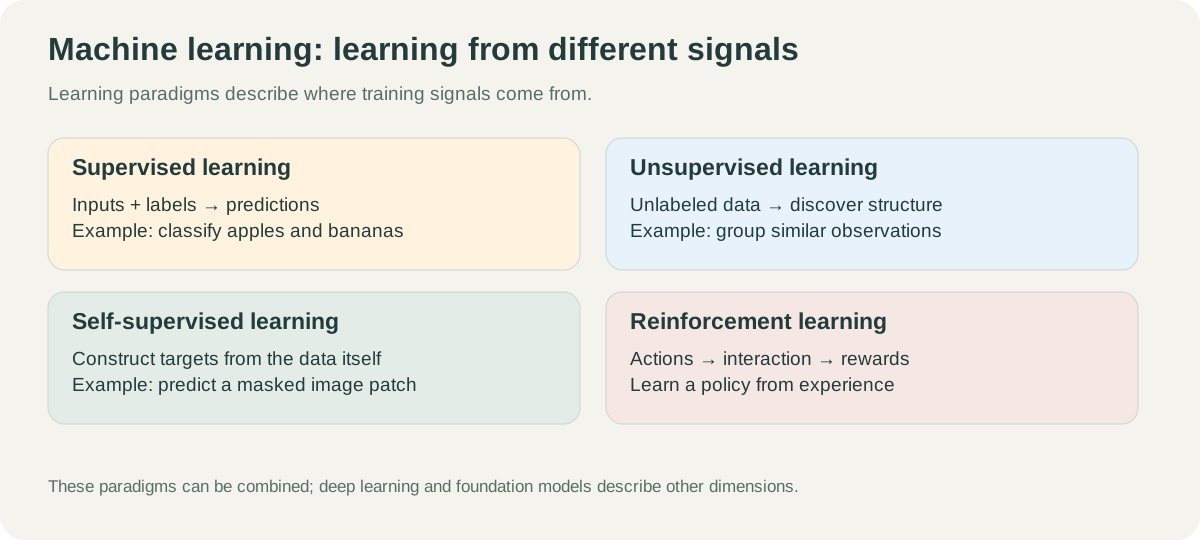
The following types of learning methods can be understood from the source of supervision signals. They are not completely mutually exclusive: the same system can do self-supervised pre-training, then supervised fine-tuning, and finally optimize decisions through reinforcement learning. Deep learning describes the model and representation learning methods, and is not in the same classification dimension as supervised learning and reinforcement learning.

2.2.1 Supervised learning (Supervised Learning)

Supervised learning is the most mature and widely used paradigm. Its training data consists of the input feature $\mathbf{x}$ and the corresponding label (Ground Truth) $y$. The goal of the model is to learn a mapping function $f: \mathbf{x} \rightarrow y$.

• core tasks: Classification (labels are discrete categories) and regression (Regression, labels are continuous values).

• Representative algorithms: linear regression, logistic regression, SVM, decision tree, and most deep neural networks.

2.2.2 Unsupervised learning (Unsupervised Learning)

The unsupervised learning data does not have the label, and the model needs to independently explore the potential structure, pattern or distribution within the data.

• Core tasks: Clustering, Dimensionality Reduction, Anomaly Detection.

• Representative algorithms: K-Means, PCA, Autoencoder, Gaussian Mixture Model (GMM).

2.2.3 Reinforcement learning (Reinforcement Learning)

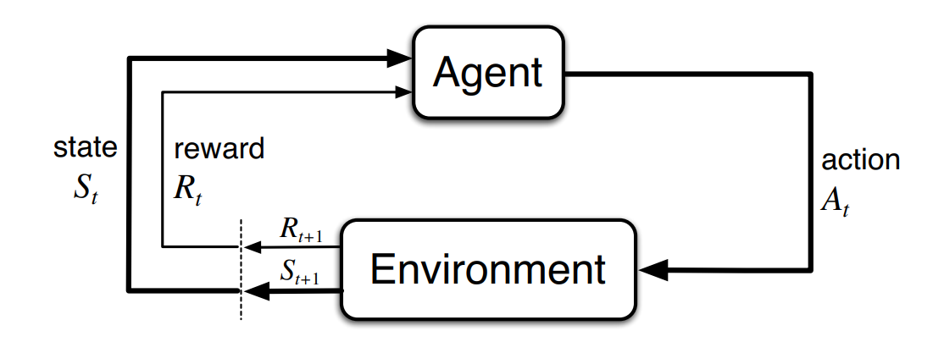
Reinforcement learning focuses on how the agent takes actions in the environment to maximize the cumulative reward. It uses rewards as feedback, which can be given immediately or delayed; training can come from online interactions or use existing interaction data for offline learning.

• Core concepts: State, Action, Reward, Policy, Value Function.

• Representative algorithms: Q-Learning, DQN, PPO, SAC.

2.2.4 Semi/Self-Supervised Learning

• Semi-supervised learning: Use a small amount of labeled data and a large amount of unlabeled data for training to reduce labeling costs.

• self-supervised learning: Constructing supervised signals from the data itself (such as predicting the next word or recovering occluded image areas) is an important training method for modern language models and many visual pretrained models.

2.3 Core elements and system architecture

A typical machine learning process usually includes the following five core elements:

1. Data (Data): The basic resource for model learning. Quality, coverage and annotation reliability directly affect the upper limit; it usually also includes data cleaning and preprocessing.

2. Feature Engineering (Feature Engineering): Convert raw data into feature vectors understandable by the model. Traditional ML strongly relies on this.

3. Model Hypothesis Space: Specifies the set of functions that the model can express, such as linear combination, tree model partitioning or neural network representation.

4. Objective Function: Defines the metric of “good” and “bad”, usually consisting of loss function (Loss Function) and regularization item (Regularization).

5. Optimization Algorithm: A strategy for solving the objective function to minimize (or maximize) parameters, such as Gradient Descent, Adam, etc.

2.4 Development history

Several representative nodes are listed below. Symbolic reasoning and machine learning have developed in parallel for a long time, and traditional methods have not lost their value due to the rise of deep learning.

period	representative node	changes in approach
1950–1980	Perceptron, expert system, and backpropagation research	From artificial rules to trainable parametric models, explore multiple routes in parallel
1990–2000	SVM, random forest, gradient boosting	Emphasis on statistical generalization, kernel methods and ensemble learning
2010–2016 years	AlexNet, ResNet, DQN, AlphaGo	Multi-layer representation learning combines large-scale data and computing resources
2017–2020 years	Transformer, BERT, GPT-3, DDPM	Self-attention, pre-training transfer and denoising generation development
2020 era	Multimodal foundation model, generative strategy, preference optimization	Study cross-task migration, generation capabilities, alignment and deployment efficiency

The main line of development is Coordinated changes in representation, objective function, data, and computing resources , not all tasks should be switched to the latest architecture.

2.5 Main challenges

Despite the fruitful results, machine learning still faces many challenges in practical implementation:

• overfitting and out-of-distribution generalization: The model performs well on the training set, but may fail after unseen data or distribution changes.

• Data quality and data leakage: Noise, bias, repeated samples, and information leakage between the training set and the test set will lead to distortion of the evaluation results.

• High dimensionality and computational cost: High-dimensional features will bring sample sparseness and computational overhead; large model training and inference also require a large amount of GPU/TPU resources.

• Interpretability and fairness: The decision-making basis of complex models is difficult to trace, and data bias may amplify unfairness between different groups.

• Evaluation and Security: Offline indicators may not represent real usage effects, and reliability, privacy, robustness and alignment still need to be continuously verified.

2.6 Key technical directions and future prospects

Machine learning continues to evolve on the frontiers of methodology and application. The following directions focus on representation, migration, adaptation, and reliability respectively, and cannot be regarded as solved problems:

• Representation Learning (Representation Learning): Automatically learn effective feature representation of data, reducing manual feature design, but still requires appropriate data processing, input representation and task design.

• Transfer Learning (Transfer Learning): Transfer the knowledge learned in one field/task to another related field/task, which greatly alleviates the problem of data scarcity.

• Meta-Learning: Also known as “learning to learn”, it aims to give the model the ability to quickly adapt to new tasks (such as Few-shot Learning).

• Cross-task generalization: Research whether the model can be transferred to new tasks, new environments and new distributions. Artificial General Intelligence (AGI) is a longer-term research goal whose achievement cannot be inferred from a single benchmark score.

• Trustworthy & Aligned AI (Trustworthy & Aligned AI): Ensure that the goals of the AI system are consistent with human values and have security, fairness and transparency.

• AI for Science: Use machine learning to solve complex computing problems in basic science fields such as physics, chemistry, biology (such as AlphaFold).

2.7 Mainstream application scenarios

Machine learning has now deeply penetrated into all aspects of the digital and physical worlds:

2.7.1 Computer Vision (CV)

• Core tasks: image classification, target detection (such as YOLO series), semantic segmentation, and image generation.

• Application: face recognition, medical image analysis, industrial defect detection.

2.7.2 Natural Language Processing (NLP)

• Core tasks: machine translation, text summarization, sentiment analysis, dialogue system.

• Application: ChatGPT and other intelligent assistants, intelligent customer service, and automatic document review.

2.7.3 Recommendation system and computational advertising

• The monetization core of Internet giants. Through technologies such as collaborative filtering and deep cross network, the matching probability between users’ historical behaviors and items is mined to achieve accurate push.

2.7.4 Robots, autonomous driving and embodied intelligence (Embodied AI)

• Combining reinforcement learning, vision and large language models allows robots to realize perception, planning, navigation and dexterous operation in complex physical environments. Such tasks also take into account observation noise, action delays, physical constraints, and distribution changes in closed-loop execution.

2.8 Mainstream data sets, evaluation benchmarks and frameworks

2.8.1 Classic data set and benchmark

Dataset	field	Characteristics and historical significance
ImageNet	CV (category)	The complete data set needs to be distinguished from the ILSVRC subset; the common ImageNet-1K refers to approximately 1.28 million training images and 1,000 classes.
COCO	CV (detection segmentation)	Released by Microsoft, it features rich multi-objective, multi-context annotation of complex scenes.
MNIST	CV (entry)	The handwritten digit recognition set is known as the “Hello World” in the field of machine learning.
GLUE	NLP	A comprehensive benchmark for evaluating natural language understanding models, driving the BERT era.

2.8.2 Mainstream tools and open source frameworks

• Scikit-learn: A traditional machine learning library under Python that provides unified interfaces for linear models, tree models, SVM, clustering, preprocessing and model evaluation.

• XGBoost / LightGBM: Gradient boosting tree framework commonly used for tabular data. The specific speed and accuracy need to be compared on the task.

• TensorFlow: Google’s open source deep learning framework, with a complete ecosystem for industrial deployment.

• PyTorch: Meta’s open source deep learning framework is widely used in research and large model training due to its dynamic graph mechanism and ease of use, and has a mature deployment ecosystem.

• Hugging Face: Provides model and data set hosting, as well as tool libraries such as transformers; when using pretrained weights, you need to check the training purpose, license and restrictions in the model card.

2.9 From data to reliable conclusions: modeling and evaluation process

Knowing the name of the algorithm is not enough. For a reproducible modeling experiment, you need to first define the task and verification method, and then optimize the model.

2.9.1 Distinguishes between fitting, optimization and generalization

Taking supervised learning as an example, given $n$ training samples, a common goal is to minimize the empirical risk and regularization terms:

\[\hat{\theta} = \arg\min_{\theta}\left[\frac{1}{n}\sum_{i=1}^{n}\ell(f_{\theta}(\mathbf{x}_i),y_i)+\lambda\Omega(\theta)\right]\]

Here, $f_\theta$ is the model, $\ell$ measures the prediction error, $\Omega$ constrains the model complexity, and $\lambda$ controls the constraint strength. optimization focuses on whether the training target can be reduced, and generalization focuses on the performance on unseen samples; low training loss does not mean that the model is reliable.

Parameters (such as linear weights) are learned by the training process; hyperparameters (such as tree depth, regularization strength, learning rate) are usually selected using the validation set. If the training and validation errors are both high, it may be due to underfitting, insufficient features, or incomplete optimization; if the training error is low but the validation error is high, overfitting and distribution differences should be investigated.

2.9.2 First divide the data and then learn the preprocessing parameters

1. Clear the forecast time point and target: The input can only contain information available at the time of actual forecast. For example, to predict whether a user churns, fields generated after churn cannot be used as features.
2. retains the test set: the training set is used for fitting, the validation set is used for parameter adjustment and threshold selection, and the test set is used for the final evaluation after the solution is determined. Repeatedly changing the model based on test results will cause the test set to lose its independence.
3. Matching deployment scenario division: Approximately independent and identically distributed classification samples can be divided randomly in a hierarchical manner; time series are divided according to time; related samples of the same user, device or robot trajectory should be divided into groups to avoid cross-collection leakage.
4. only fits the training set and preprocesses: standardization, missing value filling, feature selection and PCA all need to be fitted on the training set first, and then applied to the validation and test sets. During cross-validation, each fold must be refitted and can be managed with Pipeline.
5. records reproducible conditions: save data versions, partitions, random seeds, hyperparameters and evaluation scripts; small-sample or high variance tasks should report multi-fold or multiple running results.

Cross-validation is mainly used for model selection in the development stage and does not mean that time and grouping structure can be ignored. If you also want to use cross-validation to estimate the generalization performance of the program after parameter adjustment, nested cross-validation can be used. See scikit-learn data leakage guide and cross-validation document ].

2.9.3 Indicator must correspond to the task cost

Task	Common indicators	Interpretation points
Return	MAE, RMSE, $R^2$	RMSE is more sensitive to large errors; $R^2$ can be negative and cannot be directly ranked across different data sets
Classification	Precision, Recall, F1, confusion matrix	First clarify the positive class, threshold and false negative/false positive cost; when the class is unbalanced, you cannot just look at Accuracy
Sort by category	ROC-AUC, PR curve, Average Precision (AP)	ROC-AUC measures ranking; when positive classes are rare, you should also look at PR/AP. AP is not exactly the same as trapezoidal integral PR-AUC.
Probability prediction	Log loss, Brier score, calibration curve	Can be sorted correctly, does not mean that the output “80% probability” is consistent with the actual frequency
clustering	Silhouette coefficient, stability, domain inspection	Internal geometric indicators do not guarantee that clusters correspond to real business or semantic categories
Generation and Robot Control	Distribution indicators, manual evaluation, success rate, delay	Realistic images do not mean correct facts; low offline action error does not mean successful closed-loop tasks

For example, when the positive class only accounts for 1%, all predictions for the negative class have an Accuracy of 99%, but the Recall of the positive class is 0. The threshold should be chosen on the validation set based on the actual cost, rather than the default 0.5. For indicator definitions, see scikit-learn evaluation document .

2.9.4 Use baseline and error analysis to determine next steps

First establish naive baselines such as majority class and mean prediction, and then compare linear models, tree models or pretrained representations. If the improvement for a complex model is small, the inference latency, memory and maintenance costs should also be reported. Check which categories, time periods or groups of people the model failed, and then decide to supplement the data, change the features, adjust the target or change the architecture.

Continue to monitor input distribution, prediction quality, and feedback latency after launch. Offline testing only illustrates the performance of the model under specific data and evaluation protocols, and cannot replace post-deployment inspection.

3. Classic algorithms and representative models

This chapter organizes content by model structure and purpose. The same method may span multiple categories, for example Transformer can be used for supervised classification, self-supervised pre-training or generative modeling; AE mainly learns representations and does not automatically define sampleable generative distributions.

3.1 Core algorithm classification overview

Before delving into specific models, the following table sorts out the classic algorithm classifications and their representative models in machine learning:

Category	Representative models/techniques	Main features	Application scenarios
linear model	Linear regression, logistic regression	Simple and easy to understand, small amount of calculation and strong interpretability	House price prediction, click-through rate prediction (CTR)
Integrated learning	Random Forest, XGBoost, LightGBM	Strong robustness and excellent processing effect on tabular data	Financial risk control, search sorting
Traditional Statistics/Probability	SVM, KNN, Naive Bayes, HMM	Rigorous theory and suitable for small-sample tasks	Text classification, speech recognition, biometric information
Clustering and Dimensionality Reduction	K-Means, PCA, t-SNE	unsupervised, discover the underlying structure of data	User profiling, data compression, visualization
Deep Neural Network	CNN, RNN, LSTM, MLP	Powerful nonlinear fitting and feature extraction capabilities	Image recognition, natural language processing
Large model cornerstone	Transformer, BERT, GPT	Good at modeling long-distance dependencies and supporting large-scale pre-training	Text generation, question answering, multimodal understanding
Generative model	GAN, VAE, Diffusion Models	Learn data distribution and generate high-quality new samples	AI painting, video generation, molecular design

---

Part A · Traditional machine learning (§3.2 – §3.11) – From linear assumptions, tree partitioning, local distance to probabilistic modeling; interpretability and computational cost vary by method.

3.2 Linear regression and regularization

Core points: a straight line/hyperplane fitting data; L2 regular (Ridge) prevents overfitting, L1 regular (Lasso) comes with feature selection.

Linear Regression is the most foundation model in regression analysis, assuming a linear relationship between target variables and features. The objective function is usually to minimize the mean square error (MSE).

Intuitively understands: It is like drawing a “best fit line” on a scatter plot - the goal is to find the straight line that minimizes the sum of squares of the residuals of all points in the direction of the target variable. Regularization is equivalent to adding another constraint on the basis of “good fitting”: don’t let the weights grow too large.

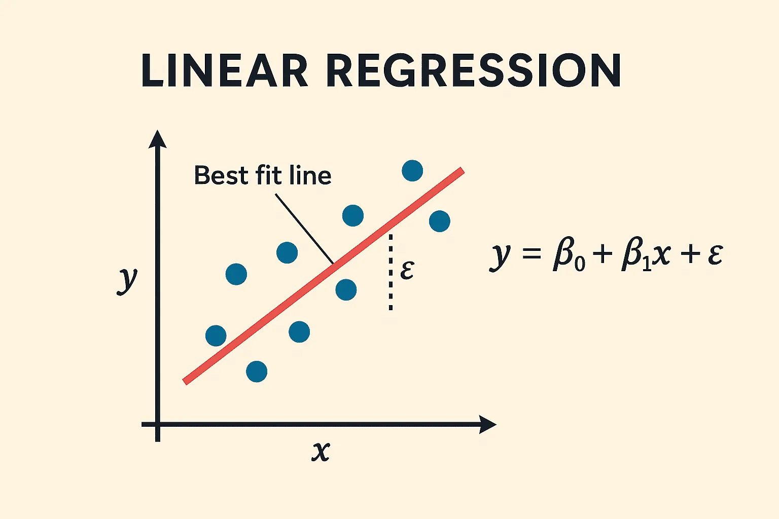
• mathematical expression: $y = \mathbf{w}^T \mathbf{x} + b$

Here, $\mathbf{w}$ is the weight vector of each feature (the coefficient size is affected by feature scale and correlation, and cannot be directly regarded as importance or causal effect), $\mathbf{x}$ is the input feature vector, and $b$ is the offset (intercept). The entire formula is “weighted sum plus a benchmark”.

• Optimization method: The closed-form solution (normal equation) can be solved directly through the least squares method, or the gradient descent method can be used for iterative optimization.

• regularization (Regularization): In order to prevent overfitting from occurring when the feature dimension is high, the regularization penalty term is often introduced in the loss function:

  • Ridge regression (L2 regularization): Add the $\lambda |\mathbf{w}|_2^2$ item to limit the sum of squares and shrinkage coefficients of parameters to alleviate estimation instability caused by multicollinearity; it is usually necessary to unify the feature scale before regularization.

  • Lasso regression (L1 regularization): Add the $\lambda |\mathbf{w}|_1$ item to limit the absolute value sum of parameters. The geometric characteristics of L1 regularization make it easy to generate sparse solutions (ie, compress some weights into 0), so it comes with a feature selection function.

Can be tried first	need attention
Features have a linear relationship with target variables	There is a complex nonlinear relationship between features and targets
Need for interpretable models	There are a lot of outliers in the data
Few features and sufficient samples	There is strong multicollinearity between features (use Ridge in this case)

3.3 Logistic Regression

Core points: The logarithmic probability is a linear function of the feature, and the binary probability is output through Sigmoid; it uses classification loss training instead of fitting a linear regression first.

Although it is named “regression”, logistic regression is mainly used for classification; here we introduce the two-classification form, and multinomial logistic regression can be used for multiple classifications. Based on linear regression, it introduces a nonlinear Sigmoid activation function to map the continuous linear output to the $(0, 1)$ interval, thus giving it probabilistic meaning.

intuitively understands: Logistic regression is a “squeezer” outside linear regression - squeezing any real number score between 0 and 1, and then treating this value directly as the “probability of belonging to the positive class”. The higher the score, the closer the probability is to 1; the lower the score, the closer the probability is to 0.

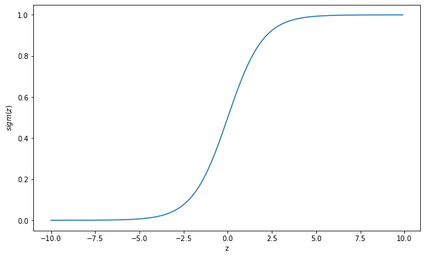
• core function:

\[P(y=1 \mid \mathbf{x}) = \sigma(\mathbf{w}^T \mathbf{x} + b) = \frac{1}{1 + e^{-(\mathbf{w}^T \mathbf{x} + b)}}\]

where $\mathbf{w}^T \mathbf{x} + b$ is the linear “raw score” and $\sigma(\cdot)$ is the sigmoid function (that “squeezer”). When the score is 0, 0.5 is output. The larger the score, the closer it is to 1, and the smaller the score, the closer it is to 0.

• loss function: Cross-Entropy Loss, derived through maximum likelihood estimation.

• Features: Low calculation cost, fast speed, output with clear probabilistic interpretation, often used in basic scenarios such as credit score cards and advertising click-through rate (CTR) estimation in financial risk control.

Can be tried first	need attention
Two classification tasks require probability output	There is a strong nonlinear relationship between features
Sparse text features, need for fast classification baseline	Complex inputs such as raw images often require extracting a suitable representation first

3.4 Decision Tree

Core points: The data is recursively divided by a series of if-then rules, which is naturally interpretable; however, a single tree has large variance and is easy to overfitting, so it needs to be pruned or integrated.

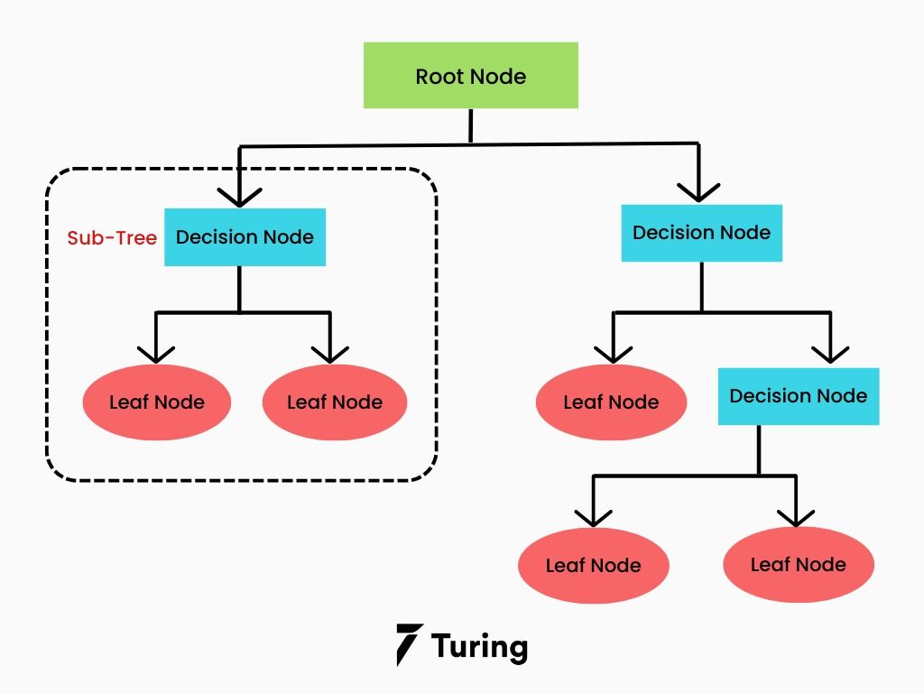
Decision trees imitate the human thinking process based on rule judgment and classify or regress data through a tree structure. Each internal node represents a conditional judgment on a certain feature, the branch represents the judgment result, and the leaf node represents the final predicted category or value.

Intuition: Just like the “guessing game” played in childhood - “Is this fruit red? → Is it → round? → Yes → Apple!” Each bifurcation point asks a question that can best distinguish the current data, narrowing down the scope layer by layer, and finally making a judgment.

• Split Criteria:

  • ID3 algorithm: Selects features based on information gain (Information Gain), and tends to select features with more values.

  • C4.5 Algorithm: Improved based on information gain rate (Gain Ratio) to alleviate the problem of information gain preferring high cardinality features.

  • CART algorithm: The classification tree uses Gini index (Gini Impurity), and the regression tree uses square error. CART is a binary tree that is the basis of many ensemble tree models.

• Advantages and Disadvantages: Shallow trees are easy to interpret and usually do not require standardization; missing value and categorical feature support depend on the specific implementation and cannot be inferred from the name “decision tree”. Deep trees are easy to overfitting, and the complexity can be controlled through the maximum depth, the minimum number of samples of leaf nodes, and pruning.

Can be tried first	need attention
Requires clear rules and shallow decision paths	It is easy to overfitting when the tree is too deep and there are too few leaf node samples.
Non-linear tabular data, usually without standardization	Category features may need to be encoded; high-precision tasks can be compared with ensemble methods

3.5 Random Forest (Random Forest)

Core points: Bagging integrates multiple separately trained decision trees in parallel, voting/average output; reduces variance, strong anti-noise, and can evaluate feature importance.

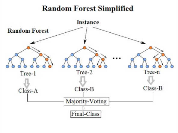
Bagging (Bootstrap Aggregating) is a parallel ensemble learning paradigm that samples data with replacement and trains multiple base learners, and then aggregates their results to reduce variance. Random forest is a representative method of bagging.

Intuition: It is equivalent to forming an “expert committee” - each expert (decision tree) only looks at some data and some features, makes their own judgment, and finally votes. Individual experts may be biased, but the collective average opinion is often more accurate and robust.

• core mechanism: By randomly sampling training samples with replacement (Bootstrap), multiple decision trees trained separately are constructed; their predictions may still be related. At the same time, when each node is split, only the optimal dividing features are selected from the features of a random subset.

• result output: The classification task produces the final result through multiple tree voting, and the regression task takes the average.

• Features: Reduces the variance of ensemble predictions by reducing the correlation between trees, but may still be overfitting. Feature importance based on node purity may be biased towards high cardinality features and can be combined with validation set permutation importance analysis; neither represents causality.

Can be tried first	need attention
Structured/tabular data, don’t want to adjust too many parameters	Very high-dimensional sparse data (such as text TF-IDF)
Nonlinear feature interaction requires a robust starting solution	Missing value support depends on implementation; the advantages and disadvantages of Boosting need to be verified

3.6 Gradient boosting tree

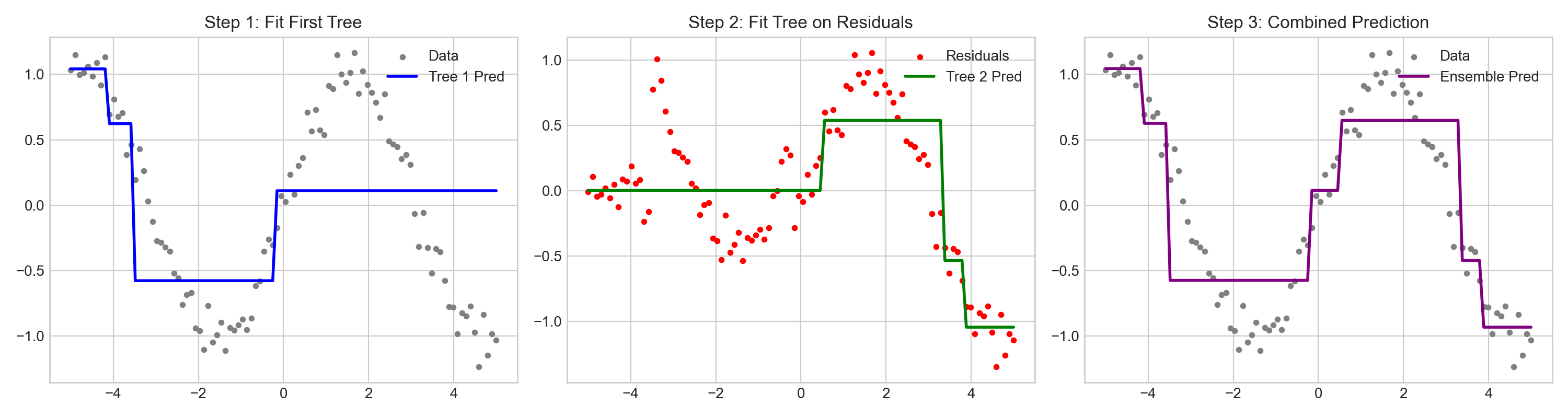
Core points: Gradient boosting fits the negative gradient of the current integrated model round by round; it is equivalent to the fitting residual under square loss. XGBoost and LightGBM provide efficient implementation.

Boosting is a serial integrated learning paradigm with the core idea of “continuous error correction”. The subsequent model focuses on the samples that the previous model predicted incorrectly, and weights and accumulates them.

Intuition: It’s like a set of questions that students got wrong - after completing the first round, the second round focuses on practicing the questions they got wrong last time, and the third round focuses on practicing the questions they got wrong last time… Each round focuses on making up for the weaknesses of the previous round, and ultimately forms a model that is strong in all aspects.

• GBDT (Gradient Boosting Decision Tree): Using the regression tree as the base learner (including when used for classification tasks), each iteration continuously approaches the true value by overfitting the negative gradient (residual under square loss) of the previous model.

• XGBoost (eXtreme Gradient Boosting): A gradient boosting framework using regularization goals and efficient tree construction methods. It not only introduces second-order derivative information (Taylor expansion) into the objective function to accelerate convergence, but also adds L1 and L2 regularization terms to control model complexity. In addition, it supports automatic processing of missing values ​​and parallel calculation of features, and has long been used as a strong baseline in Kaggle tabular data competitions.

• LightGBM: A more efficient Boosting framework launched by Microsoft. By introducing the histogram-based decision tree algorithm, one-sided gradient sampling (GOSS), and exclusive feature bundling (EFB), the training efficiency in some tasks is improved; whether these technologies are enabled and their effects depend on the configuration and data.

Can be tried first	need attention
Structured tabular data, pursuit of accuracy	Unstructured data such as images/text
Data contains missing values (XGBoost automatically handles)	Very few training samples, easy to overfitting

3.7 K nearest neighbor algorithm (KNN)

Core points: Lazy learning - no training, only memory, vote/average based on the nearest K neighbors when predicting; simple and intuitive but slow inference, sensitive to scale, and affected by the disaster of dimensionality.

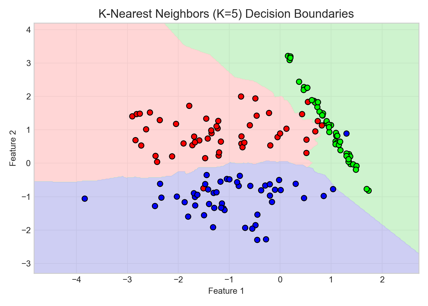
KNN is a typical “Lazy Learning” algorithm. It does not fit an explicit parameterized prediction function and mainly saves training samples. In actual implementation, it is also possible to build a nearest neighbor search index.

Intuition: It’s like asking for directions in a strange city - without relying on any map (no training required), just ask the nearest $K$ passers-by around you and get the opinion of the majority. It completely relies on the simple assumption that “birds of a feather flock together and people flock together”.

• prediction mechanism: When predicting, calculate the distance (such as Euclidean distance, Manhattan distance) between the test sample and all training samples, and find the nearest $K$ samples in the feature space.

• Decision rule: Majority voting is used for classification tasks and the mean is used for regression tasks. A distance weighting mechanism can be introduced, the closer the distance, the greater the weight.

• Disadvantages: Brutal search requires comparing all training samples; tree index can speed up some low-dimensional tasks, but the benefits are limited in high dimensions. Distance is affected by feature scale, and a suitable metric should usually be standardized or designed.

Can be tried first	need attention
Small data set, rapid prototyping	Large data sets (prediction speed decreases linearly with sample size)
Irregular data distribution and non-spherical category boundaries	High-dimensional data (seriously affected by the curse of dimensionality)

3.8 Naive Bayes and Hidden Markov Model

Core points: Naive Bayes assumes independent feature conditions, fast training, and good text classification effect; the “hidden state + observation” of HMM modeling sequence is suitable for explicitly describing the relationship between state transition and observation generation.

Naive Bayes

Naive Bayes is a classification algorithm based on Bayes’ theorem, which makes an extremely strong but very efficient “naive” assumption—— Features are conditionally independent of each other .

Intuition: Just like a judge judging a case based on multiple “independent clues” - assuming that each clue does not affect each other, multiply the support of each clue, and choose the conclusion with the highest score. This independence assumption is rarely true in reality, but it is often sufficient in practice.

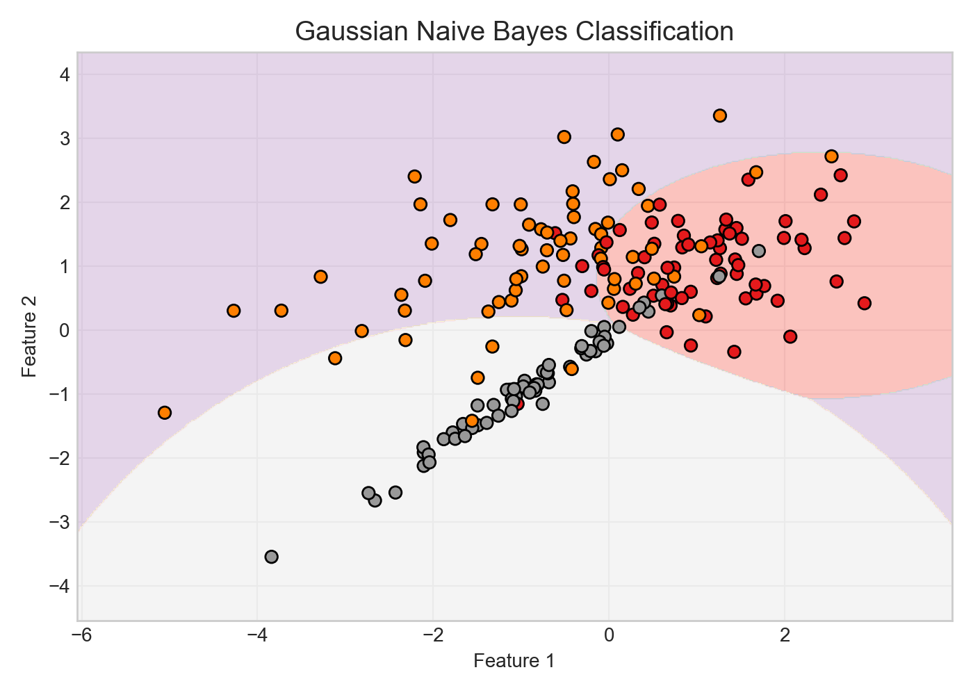
• Bayes’ theorem: Given the sample characteristics $\mathbf{x} = (x_1, x_2, \dots, x_n)$, the posterior probability is:

\[P(y \mid \mathbf{x}) = \frac{P(\mathbf{x} \mid y) \cdot P(y)}{P(\mathbf{x})}\]

formula interpretation: $P(y \mid \mathbf{x})$ is “the probability that the sample belongs to the category $y$ after seeing the feature $\mathbf{x}$” (posterior); $P(\mathbf{x} \mid y)$ is “$y$” “The likelihood” (likelihood) that a class sample will have this set of features; $P(y)$ is the prior probability of the class. The denominator $P(\mathbf{x})$ is the same for all categories and can be ignored when classifying.

• Naive hypothesis: Assuming that each feature is conditionally independent under a given category, the joint probability is decomposed into the product of the probabilities of each feature:

\[P(\mathbf{x} \mid y) = \prod_{i=1}^n P(x_i \mid y)\]

• Classification decision: Select the category that maximizes the posterior probability, that is:

\[\hat{y} = \arg\max_y P(y) \prod_{i=1}^n P(x_i \mid y)\]

• Features: Although the conditional independence assumption is rarely strictly true in reality, Naive Bayes can often achieve amazing results in text classification (spam filtering, sentiment analysis), and the training speed is extremely fast and suitable for very large-scale data.

Can be tried first	need attention
Text classification (spam filtering, sentiment analysis)	There is a strong correlation between features
Fast baselines with very few samples	Requires precise probabilistic calibration

Hidden Markov Model (HMM)

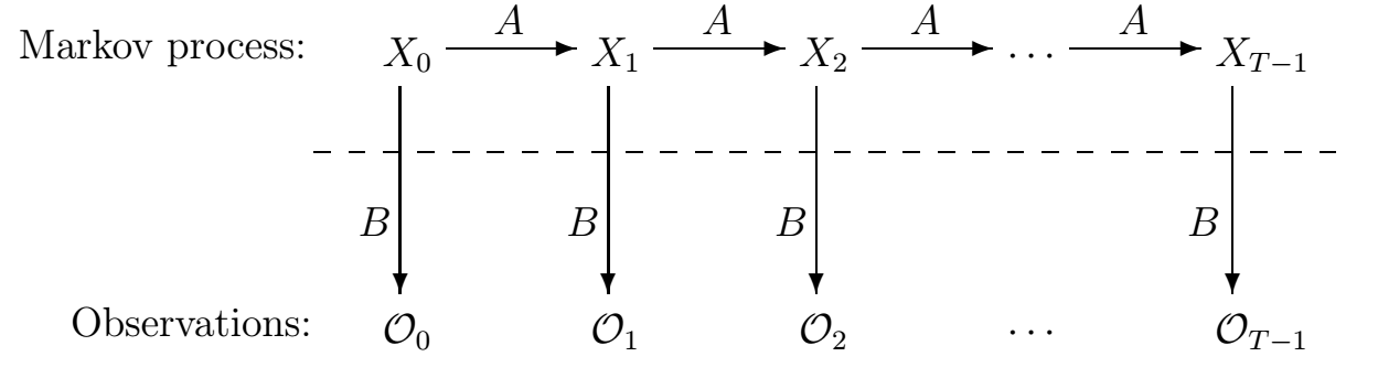
HMM is a probabilistic graphical model for processing sequence data, containing an unseen hidden state sequence and a visible observation sequence.

Intuition: Just like a doctor infers the internal cause (viral infection or bacterial infection, which is an invisible “hidden state”) by observing symptoms (fever, cough, which are visible “observations”). The cause itself is invisible, but the most likely sequence of causes can be deduced from the sequence of symptoms.

• Two core assumptions:

  • Markov hypothesis: The current hidden state $s_t$ only depends on the previous hidden state $s_{t-1}$, which is $P(s_t \mid s_1, \dots, s_{t-1}) = P(s_t \mid s_{t-1})$.

  • observation independence hypothesis: The current observation $o_t$ only depends on the current hidden state $s_t$, that is, $P(o_t \mid s_1, \dots, s_t) = P(o_t \mid s_t)$.

• Three basic questions:

  1. Evaluation question: Given model parameters, calculate the probability of a certain observation sequence (forward-backward algorithm).

  2. decoding problem: Given an observation sequence, find the most likely hidden state sequence (Viterbi algorithm).

  3. Learning problem: Estimating model parameters from observational data (Baum-Welch/EM algorithm).

• application scenarios: early speech recognition, part-of-speech tagging (POS tagging), gene sequence analysis. Although many speech and NLP tasks turn to deep models, HMMs are still valuable in sequence problems with state interpretation, limited data, and clear domain constraints.

3.9 Support Vector Machine (SVM)

Core points: Find the classification hyperplane with the largest interval; the kernel technique models nonlinear boundaries through implicit feature mapping, but does not guarantee that the data is separable, nor can it eliminate statistical dimensionality problems.

Before deep learning was widely used, SVM (Support Vector Machines) was an important baseline in small-sample and high-dimensional classification tasks.

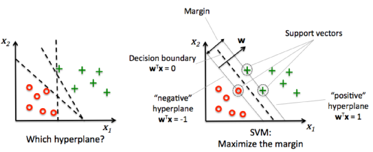
Intuition: Imagine two groups of points distributed on the plane. SVM needs to draw a line in the middle so that the two groups of points are as far away from this line as possible - just like digging a “moat” as wide as possible between the two armies. The optimal boundary is determined by the support vector and its coefficient; in the case of soft margin, some samples are also allowed to enter the interval or be misclassified.

• core idea : Try to find a hyperplane in the feature space so that samples of different categories are not only correctly separated, but also Geometric Margin Maximization . This pursuit of “maximum interval” gives SVM extremely strong generalization capabilities.

• support vector: The training samples with non-zero coefficients in the dual problem are called support vectors. The support vectors of soft-margin SVM may also fall within the margin or even be misclassified.

• Kernel Trick : When the data is linearly inseparable in the original space, SVM cleverly implicitly maps low-dimensional features to high-dimensional (or even infinite-dimensional) space through kernel functions (such as linear kernel, polynomial kernel, Gaussian RBF kernel), thereby constructing nonlinear decision boundaries. The kernel technique eliminates the need to explicitly construct high-dimensional features, but still has kernel matrix calculation costs and overfitting risks.

Can be tried first	need attention
Small sample, high-dimensional data (text, gene features)	Large-scale kernel SVM is computationally and storage expensive; linear SVM can use more scalable solvers
Feature Dimension » Sample Number Scenario	Probability output is required (SVM itself does not output probabilities)

3.10 K-Means clustering

Core points: unsupervised clustering classic baseline, alternately updates “sample allocation → centroid position” to convergence; requires a preset K value, is only good at spherical clusters, and is sensitive to initial values and outliers.

The most classic and widely used unsupervised clustering algorithm.

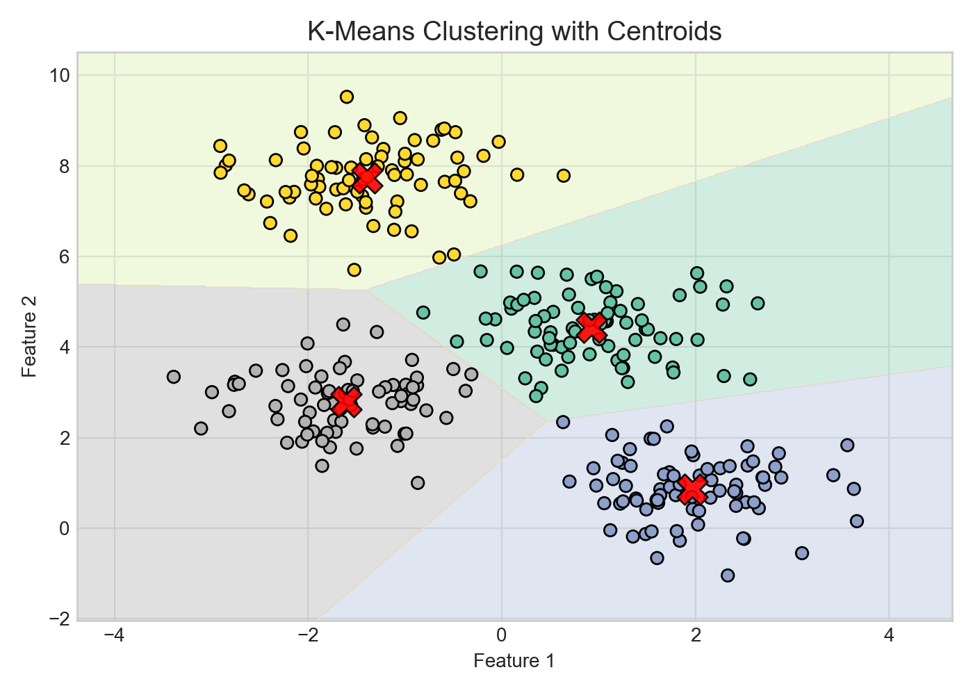
intuitively understands: It’s like choosing $K$ squad leaders - first randomly assign a squad leader, and all students in the class will approach the nearest squad leader; then reselect the center of each group as the new squad leader…and repeat this until the squad leader’s position is stable.

• algorithm flow:

  1. Randomly initialize $K$ cluster centers (Centroids).

  2. Traverse all samples and assign them to the nearest cluster center.

  3. According to the assigned clusters, the centroid of each cluster (that is, the mean of all samples) is recalculated and the cluster center is updated.

  4. Repeat steps 2 and 3 until the cluster centers no longer change significantly (converge) or the maximum number of iterations is reached.

• Advantages and Disadvantages: The algorithm is simple and efficient. The time complexity of a typical Lloyd iteration is $O(nKdi)$ ($d$ is the feature dimension, $i$ is the number of iterations); but it is sensitive to the selection of initial values and outliers, and $K$ must be specified in advance. value, prefers clusters with approximately spherical shapes and similar scales, and is difficult to process data with complex manifold distributions.

Can be tried first	need attention
The data distribution is close to spherical and the sizes of each cluster are similar.	Cluster shapes are irregular (use DBSCAN instead)
Quickly obtain clustering results and user portrait grouping	Scenarios where the $K$ value is difficult to determine

3.11 Principal Component Analysis (PCA) and t-SNE

Core points: PCA does linear dimensionality reduction and preserves global variance; t-SNE does nonlinear dimensionality reduction and preserves local manifold structure, which is the first choice for 2D/3D visualization.

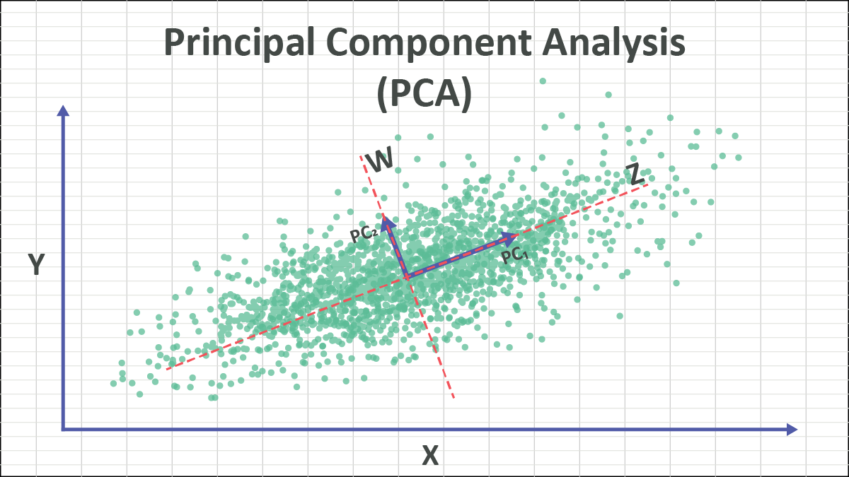
• Principal Component Analysis (PCA): A classic linear dimensionality reduction method. The core idea is to project the potentially relevant original high-dimensional features into a new orthogonal coordinate system through orthogonal transformation. These new coordinate axes (principal components) are arranged according to the size of the data variance. Retaining the first few principal components with the largest variance can minimize the squared reconstruction error under a given linear subspace dimension; the direction of high variance does not necessarily contain the most beneficial information for downstream prediction.

  intuitively understands: It’s like taking a photo of a three-dimensional object - choose a “shooting angle” that best retains information, so that the projected 2D image has the largest amount of information (maximum variance). PCA automatically finds this optimal angle.

• t-SNE (t-Distributed Stochastic Neighbor Embedding): A nonlinear dimensionality reduction algorithm mainly used to map high-dimensional data to 2D or 3D space for visualization. It expresses similarity by converting the Euclidean distance between data points into conditional probabilities, and uses t-distribution to alleviate the “crowding problem” when high-dimensional space is mapped to low-dimensional. It can excellently maintain the local manifold structure and intra-class aggregation characteristics of the data.

  Intuitively understands: It is like flattening a ball of high-dimensional “plasticine” on the table. Try to keep the points that are close to each other still close after flattening, and the points that are far away do not have the same strong distance to maintain constraints. Therefore the inter-cluster distances, areas and gaps in the graph cannot be directly interpreted as the real structure of the original space.

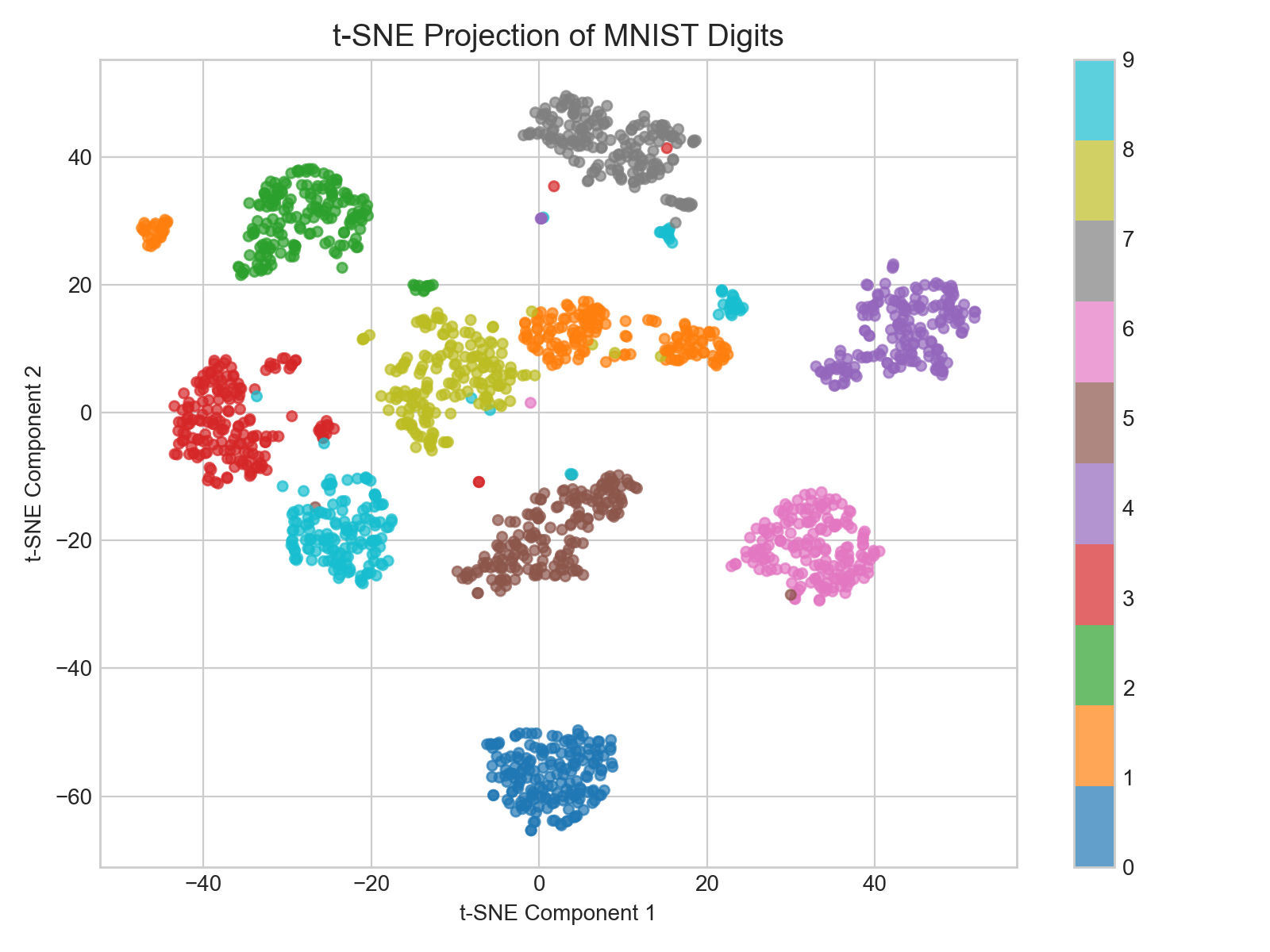
t-SNE is sensitive to hyperparameters such as random initialization and perplexity, and cannot prove the classification effect or discover “real categories” solely by clustering in the graph; it is mainly an exploration tool and should not directly replace the generalizable dimensionality reduction process in prediction tasks. See scikit-learn manifold learning document .

---

Part B · Deep learning basics (§3.12 – §3.15) - Learn representations through multi-layer nonlinear transformations, using backpropagation to calculate gradients.

This chapter only outlines the core context; activation functions, optimizers, normalization, regularization and training techniques can be further read: “Review of deep learning” .

3.12 Multilayer Perceptron (MLP) and Backpropagation

Core points: fully connected layer + nonlinear activation + backpropagation; strong function expression ability under appropriate conditions; expression ability, trainability and generalization ability need to be judged separately.

Deep learning (Deep Learning, DL) extracts high-order features of data through multi-layer nonlinear transformation. Multilayer Perceptron (MLP) is the most basic feedforward neural network and the starting point for understanding all deep networks.

Intuitively understands: Just like an assembly line - the raw materials (input features) go through multiple processing steps (hidden layers), and each step uses an activation function to introduce “bends”, allowing the assembly line to process any complex shape (function). The deeper the layer, the more complex the “processing logic” that can be expressed.

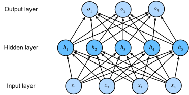
• structure: consists of an input layer, one or more hidden layers and an output layer, with full connections between layers. Each neuron receives a weighted sum of the outputs of the previous layer and is processed by a nonlinear activation function. The calculation of a single layer can be expressed as:

\[\mathbf{h} = \sigma(\mathbf{W}\mathbf{x} + \mathbf{b})\]

in $\mathbf{W}$ is the weight matrix of this layer (the strength of each connection), $\mathbf{x}$ is the output of the previous layer, $\mathbf{b}$ is the bias vector, $\sigma$ is a nonlinear activation function—— Without it, multi-layer linear transformation is equivalent to single-layer linear transformation, and the network loses the meaning of depth. .

• Activation function: The introduction of nonlinearity is the key to deep networks - without an activation function, multi-layer linear transformation is equivalent to a single layer. Common activation functions:

  • Sigmoid: $\sigma(x) = \frac{1}{1+e^{-x}}$, output $(0,1)$, easy gradient disappears.

  • Tanh: Output $(-1,1)$, zero centralization, but still with vanishing gradient problem.

  • ReLU: $\text{ReLU}(x) = \max(0, x)$, which is simple to calculate and alleviates vanishing gradients, is one of the commonly used activation functions. Negative interval gradients of zero may result in persistent inactivation of neurons; Leaky ReLU, GELU, etc. are other common choices.

• Universal Approximation Theorem: Under conditions such as appropriate activation functions, a sufficiently wide single hidden layer network can arbitrarily approximate a continuous function in a compact domain. This theorem does not guarantee that the required width is acceptable, nor does it guarantee that it can be trained with limited data or that generalization is good; deep structures have higher expression efficiency for certain functions.

• Backpropagation: The cornerstone of neural network training.

  1. Forward propagation: The input data is calculated layer by layer to obtain the predicted output and loss $\mathcal{L}$.

  2. Backpropagation: Based on the calculus-based chain rule, the gradient of the loss for each parameter is calculated layer by layer in reverse from the output layer. For example, the gradient for weight $W_{ij}$: $\frac{\partial \mathcal{L}}{\partial W_{ij}} = \frac{\partial \mathcal{L}}{\partial \hat{y}} \cdot \frac{\partial \hat{y}}{\partial h} \cdot \frac{\partial h}{\partial W_{ij}}$.

  3. parameter update: Use gradient descent algorithm to update parameters, such as SGD: $\mathbf{W} \leftarrow \mathbf{W} - \eta \frac{\partial \mathcal{L}}{\partial \mathbf{W}}$.

• Commonly used optimizer:

  • SGD + Momentum: Accumulate historical gradients to reduce directional oscillation and improve the convergence speed of some optimization problems.

  • Adam: Adaptive learning rate optimizer, which combines the advantages of Momentum and RMSProp and is suitable for many deep learning tasks; whether it is better than SGD depends on the task and parameter adjustment.

Can be tried first	need attention
Getting started with deep learning for general tabular data	Image (using CNN), sequence (using RNN/Transformer)
Classification/regression tasks after feature engineering improvement	The amount of data is very small (large number of parameters, easy to overfitting)

3.13 Convolutional Neural Network (CNN)

Core points: Local receptive field + weight sharing + pooling, born for grid data such as images; ResNet residual connection allows the network to be trained to hundreds of layers, which is the cornerstone of computer vision.

CNN is a neural network architecture designed specifically for processing grid-like topological data (such as the 2D pixel grid of an image) and is a cornerstone of the field of computer vision.

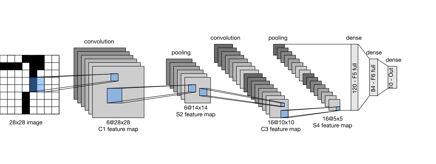
Intuition: The convolution kernel of CNN is like a sliding “magnifying glass”, scanning the image area by area - identifying edges and colors in the shallow layer, texture and shape in the middle layer, and combining high-level semantics such as “ears” and “eyes” in the deep layer. Layers of abstraction, finally recognizing “this is a cat”.

• Core mechanism:

  • local receptive field and convolution kernel: Use small filters (convolution kernels) to slide on the input feature map to extract local features (such as edges, textures), greatly reducing the amount of parameters.

  • Weight sharing: The same convolution kernel traverses the entire image, making the model have translational equivariance.

  • Pooling layer (Pooling): Such as max pooling, used for downsampling and local aggregation, which can improve tolerance to small displacements, but does not guarantee strict translation invariance. Striding and boundary processing also affect the equivariant properties of the network.

• Classic architecture: LeNet-5 (early handwritten digit recognition), AlexNet (detonating deep learning), VGG (stacked small convolution kernels), ResNet (introducing residual connections to solve the problem of deep network degradation, with a depth of up to hundreds of layers).

Can be tried first	need attention
Grid data such as images and videos	Pure sequence/text data (use Transformer instead)
Requires translation invariance and local feature extraction	Very small amount of data (can be mitigated by transfer learning)

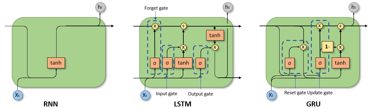
3.14 Recurrent Neural Network (RNN & LSTM/GRU)

Core points: The hidden state gives the network time memory; LSTM/GRU uses a gating mechanism to alleviate the gradient problem in long-distance dependent learning, and was the main force in sequence modeling before the emergence of Transformer.

The recurrent neural network family has experienced the evolution of RNN → LSTM → GRU. LSTM and GRU are two different gating structures. The method proposed later is not necessarily better on every task.

RNN — basic recurrent structure

RNN is specially used to process variable-length sequence data such as text, speech, and time series. Unlike ordinary neural networks, it retains a “hidden state” when processing each time step and passes it to the next step, giving the network temporal memory.

Intuition: Just like a reader who memorizes while reading - each step merges “current input + previous step memory” into a new memory and passes it to the next step.

• hidden state mechanism: The calculation of each time step is $h_t = \tanh(W_h h_{t-1} + W_x x_t + b)$, where $h_{t-1}$ is the hidden state of the previous step and $x_t$ is the current input.

• Difficulty in long-distance dependencies: Backpropagation in the time dimension (BPTT) requires multiple consecutive gradients, which is prone to vanishing gradients or explosion, making it difficult for basic RNN to stably learn distant dependencies.

LSTM — gated memory

The Long Short-Term Memory network provides a more direct gradient propagation path and alleviates the difficulty of long-term dependent learning by introducing cell state (Cell State) and three gating mechanisms. However, it does not guarantee that the gradient will never disappear or explode.

Intuition: LSTM Three switches are installed for the memory - forgetting gate determines “which old memories can be deleted”, input gate determines “which new information is worth remembering”, output gate determines “which part of the memory is now output to the outside world”. The cell state is like a highway, and the degree of information retention is determined by the gate value.

• forget gate: $f_t = \sigma(W_f [h_{t-1}, x_t] + b_f)$, output 0~1 determines which of the old cell states are retained (0 = completely forgotten, 1 = completely retained).

• input gate: $i_t = \sigma(W_i [h_{t-1}, x_t] + b_i)$, determines which new information is written; the candidate content is \(\tilde{C}_t = \tanh(W_C [h_{t-1}, x_t] + b_C)\).

• cell status update: \(C_t = f_t \odot C_{t-1} + i_t \odot \tilde{C}_t\), selective new information is added after the old memory is selectively forgotten ($\odot$ is element-wise multiplication).

• output gate: $o_t = \sigma(W_o [h_{t-1}, x_t] + b_o)$, the final output is $h_t = o_t \odot \tanh(C_t)$, which determines what is output to the current step.

GRU — lightweight improvements

Gated Recurrent Unit (Cho et al. 2014) is a simplification of LSTM: three gates are merged into two, independent cell states are canceled, and there are usually fewer parameters for the same input and hidden state dimensions. The specific speed and effect still need to be measured.

intuitively understands: GRU combines the forget gate and the input gate into a update gate (“how many old ones should be retained and how many new ones should be introduced”), and uses reset gate to control the impact of historical information. The structure is simpler and reasoning is faster.

• reset gate: $r_t = \sigma(W_r [h_{t-1}, x_t])$, controls the impact of the previous hidden state on the candidate state, which is equivalent to “restart” when close to 0.

• update gate: $z_t = \sigma(W_z [h_{t-1}, x_t])$, which simultaneously plays the role of forgetting gate and input gate: \(h_t = (1-z_t) \odot h_{t-1} + z_t \odot \tilde{h}_t\).

• Selection Suggestions: When the sequence is long or stronger memory capacity is required, try LSTM; when pursuing training speed or when resources are limited, try GRU first. The effect of the two depends on the task and data. It is recommended to compare through the validation set.

Can be tried first	need attention
Short to medium length sequences (time series prediction, speech frames)	Very long sequences (Transformer parallel processing is more efficient)
Resource constraints require lightweight real-time inference (GRU preferred)	Need to capture distant context in text

3.15 Transformer Architecture

Core points: With Self-Attention as the core, parallel modeling of global long-distance dependencies; Transformer has become the infrastructure of many languages, multi-modal and generative models.

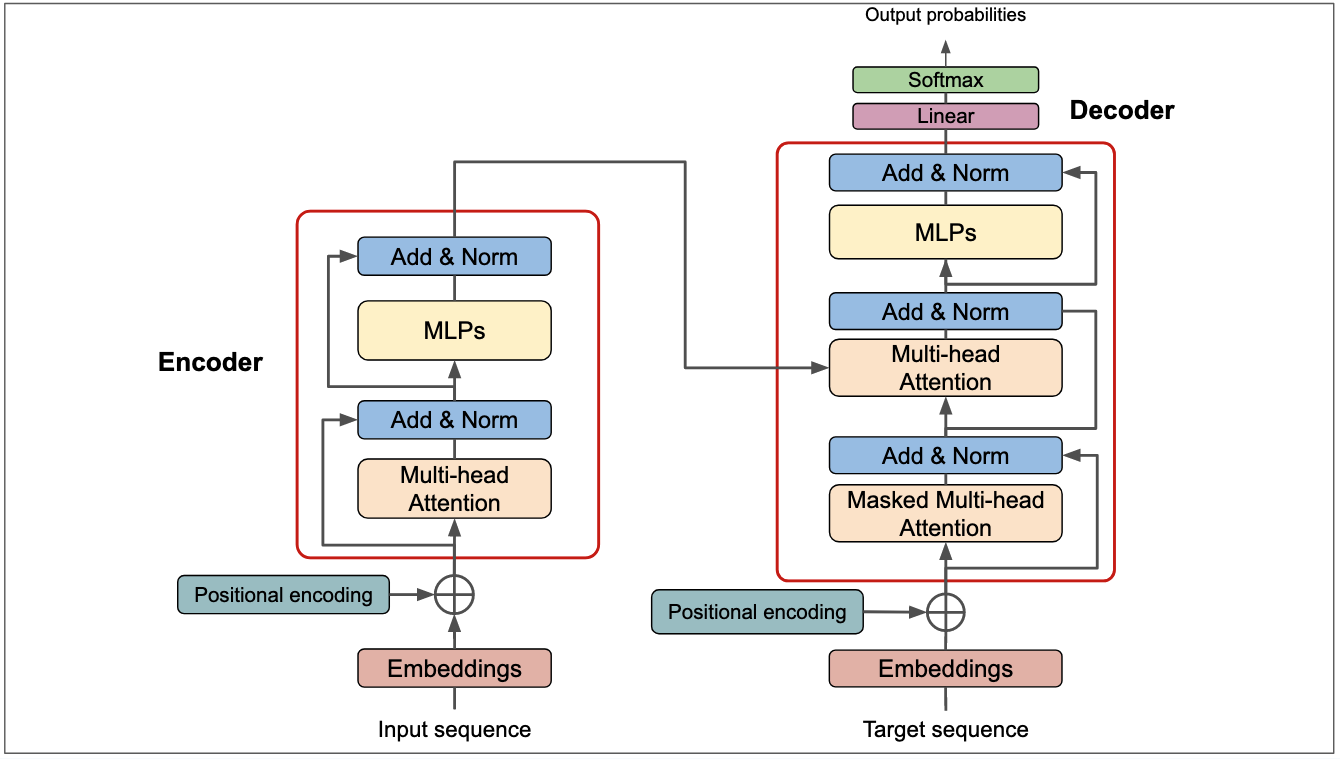
Transformer (Vaswani et al., 2017, “Attention Is All You Need”) takes self-attention and feed-forward networks as its core, gets rid of the serial dependence of cyclic structures, and has become an important architecture of many modern foundation models.

Intuition: Transformer is like a “global conference room” - each token can interact directly with the position allowed by the mask (self-attention), and there is no need to rely on “messaging” to transmit information like RNN. Therefore, it can process in parallel and efficiently capture context dependencies at any distance.

Self-Attention mechanism (Self-Attention)

Global self-attention without causal restrictions allows each element in the sequence to focus on other positions; causal self-attention can only focus on the current position and the previous position, and calculate the association weight between them, thereby capturing global long-distance dependencies in parallel.

• The input sequence is generated through three linear transformations: Query ($Q$), Key ($K$), Value ($V$) matrix.

• The attention weight is calculated by the dot product of $Q$ and $K$, and then weighted by Softmax normalization $V$:

\[\text{Attention}(Q, K, V) = \text{softmax}\left(\frac{QK^T}{\sqrt{d_k}}\right)V\]

formula interpretation: $Q$ = “What am I looking for”, $K$ = “What keywords can I provide”, $V$ = “My actual content”. $Q \cdot K^T$ calculates the correlation score of each pair of tokens and divides it by $\sqrt{d_k}$ to prevent the Softmax gradient from disappearing due to excessive scores. Finally, $V$ is weighted and summed to obtain a new representation of each token that incorporates contextual information.

Multi-Head Attention

Split $Q, K, V$ into $h$ independent “heads”, each head calculates attention in different subspaces, and finally splices:

\[\text{MultiHead}(Q, K, V) = \text{Concat}(\text{head}_1, \dots, \text{head}_h)W^O\]

Different heads can focus on different levels of relationships (grammatical relationships, semantic relationships, positional relationships, etc.) at the same time, greatly improving expression capabilities.

Transformer Block Structure

Basic Encoder Block and common Decoder-only Block include the following two types of sub-layers, which are combined with residual connection and LayerNorm to improve training stability; the Decoder of the original Encoder-Decoder model also includes cross-attention:

1. Multi-head self-attention layer: Capture the dependencies between tokens.
2. Feedforward Network (FFN): Two layers of linear transformation sandwich an activation function, and each position is independently transformed nonlinearly: $\text{FFN}(x) = W_2 \cdot \text{ReLU}(W_1 x + b_1) + b_2$.

Positional Encoding

Without position encoding and order-dependent masks, the self-attention pair arrangement is equivariant: scrambling the input will cause the output to be rearranged in the same way, rather than the output being completely unchanged. Therefore, it is usually necessary to add location information to distinguish the order. The original solution used sine/cosine functions to encode absolute position; subsequently, relative position encoding schemes such as RoPE (rotational position encoding, adopted by LLaMA series) and ALiBi were developed.

Encoder-Decoder architecture

• Encoder: $N$ Blocks are stacked, and the input tokens can follow each other in both directions, which is suitable for “understanding” tasks (such as source language encoding for machine translation).
• Decoder: The same $N$ Blocks, but the self-attention layer adds causal mask (Causal Mask) - each token Only the content before it can be seen (autoregressive generation); and cross attention layer, $Q$ from Decoder, and $K, V$ from Encoder are added to realize attention to the source language.

Why Transformer can replace RNN

RNN must be processed serially in time steps ($O(n)$ serial dependency) and cannot fully utilize GPU parallelism; Self-Attention calculates the relationship of all token pairs in parallel at once (training complexity $O(n^2 d)$), which facilitates parallel processing of sequences in training and shortens the information path between remote locations. However, deep Transformers may still have optimization and gradient problems; standard autoregressive inference still proceeds according to the generation step, and attention also has a secondary computational cost. Original paper discusses these architectural differences.

Can be tried first	need attention
Long sequences, need global context (NLP, multi-modal)	GPU memory consumption is large when the sequence is very long ($O(n^2)$, requires optimization such as Flash Attention)
Large-scale pre-training scenarios with sufficient data volume	Very small data set (weak inductive bias, not as fast as CNN convergence)

---

Part C · Pre-training large model paradigm (§3.16) - Transformer × massive unlabeled corpus, the new paradigm of “pre-training + fine-tuning/Prompt” has completely changed NLP and gave birth to the era of large models.

3.16 BERT and GPT series model paradigms

Core points: BERT uses a bidirectional Encoder to be good at understanding tasks (classification, extraction); GPT uses an autoregressive Decoder to be good at generation, and can improve interactive behavior by combining instruction fine-tuning and preference optimization.

Here we compare two representative pre-training methods. They are not a strict demarcation between “understanding” and “generating”: Decoder-only models can also do classification, and Encoder-Decoder models (such as T5) provide another way of organizing.

Intuition: BERT is like doing a fill-in-the-blank question - randomly remove a few words from the sentence and let the model guess it based on the context, forcing it to understand the two-way context. GPT is like continuing a story - giving you the first half, word by word, learning language rules through a large number of sequence predictions, and can be adapted to tasks such as question and answer, coding, etc.; these abilities require specific evaluation.

BERT — Bidirectional Encoder Paradigm

BERT (Bidirectional Encoder Representations from Transformers, Google 2018) adopts the Encoder part of Transformer. The core innovation lies in bidirectional context modeling.

• pre-training task:

  • Masked Language Model (MLM): The token of 15% is randomly selected as the prediction target; in these positions, 80% is replaced with [MASK], 10% is replaced with a random token, 10% Leave it as is. The model predicts the original token based on the bidirectional context. The proportion is for the “selected position”, not the entire input. BERT’s original paper gives the specific process.

  • Next sentence prediction (NSP): Determine whether two sentences are contextually continuous and help the model learn inter-sentence semantics.

• usage paradigm - “pre-training + fine-tuning”: first pre-train on large-scale unlabeled corpus, and then fine-tune with a small amount of labeled data on specific downstream tasks. BERT has significantly set records on benchmarks such as GLUE and SQuAD, defining the standard paradigm in the NLU era.

• Limitations: MLM’s [MASK] tag does not exist during inference, resulting in a distribution mismatch between pre-training and inference (Pretrain-Finetune Discrepancy); and the Encoder architecture is not good at text generation tasks.

• follow-up development: RoBERTa (removing NSP, larger data and longer training), ALBERT (parameter sharing compression), DeBERTa (decoupling attention) and other further optimizations.

GPT — Autoregressive decoder paradigm

GPT (Generative Pre-trained Transformer, OpenAI) uses the Decoder-only structure with causal self-attention (usually without the cross-attention to the Encoder in the original translation model), and generates text token by token through autoregression.

• pre-training task - predict the next token: given the previous text $x_1, x_2, \dots, x_{t-1}$, predict the next token $x_t$. Training usually minimizes the negative log-likelihood, which is equivalent to maximizing the sequence log-likelihood:

\[\mathcal{L}_{\mathrm{NLL}} = -\sum_{t=1}^{T} \log P(x_t \mid x_1, \dots, x_{t-1}; \theta)\]

The Causal Mask is used to ensure that only the previous token can be seen at each position to ensure autoregressive constraints.

• Scaling Laws and Emergent Ability: The language model loss exhibits an empirical scaling relationship with parameters, data and calculation scale within a certain experimental range, but this cannot guarantee that all task capabilities can be improved simultaneously. “Emergence” is also affected by evaluation metrics: discrete scores may show continuous improvements as sudden jumps, and should be interpreted in conjunction with the task, model family, and measurement method. See Kaplan et al. and Study on emergent measurement.

• Historical representative model (used to understand method evolution, not a complete product list):

model	Parameter quantity	key breakthrough
GPT-1	117 million	Verified the feasibility of “unsupervised pre-training + supervised fine-tuning”
GPT-2	1.5 billion	Demonstrates zero-shot capabilities, and the quality of text generation arouses social concern
GPT-3	175 billion	In-context Learning, few-shot capabilities are amazing and no fine-tuning is required
GPT-4	Undisclosed	Multi-modality (text + image input), RLHF alignment, stronger reasoning capabilities

• Instruction fine-tuning and preference optimization: Supervised fine-tuning (SFT) learning demonstration answer; the typical RLHF process reuses preference data to train the reward model, and uses methods such as PPO to optimize the strategy. DPO directly uses preference pairs to optimize the language model, without the need to separately train an explicit reward model or run PPO during the fine-tuning process. Both rely on the quality of feedback and cannot guarantee factual accuracy or eliminate all risks. See InstructGPT and DPO.

Comparison of two paradigms

Dimensions	BERT(Encoder)	GPT(Decoder)
attention direction	Bidirectional (full context)	One-way (see the previous article only)
Pre-training tasks	Masked language model (fill in the blank)	Next token prediction (continuation)
good at task	Understanding classes (classification, extraction, matching)	Generative classes (conversation, writing, reasoning)
Use paradigm	Pre-training + fine-tuning	Pre-training + Prompting/In-context Learning
Selection considerations	Suitable for fixed output, representation extraction and task fine-tuning	Suitable for open-ended output; still needs to evaluate cost, illusion, and task performance

---

Part D · Generative model (§3.17 – §3.20) - From adversarial game (GAN) to probabilistic modeling (VAE) to denoising diffusion (Diffusion), AI moves from “understanding data” to “creating data”.

3.17 Generative Adversarial Network (GAN)

Core points: Generator and discriminator game confrontation, G for fraud, D for fraud; sampling usually only requires one generator forward, but the training may be unstable and there is a risk of model collapse.

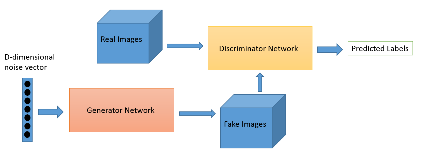
GAN (Generative Adversarial Network) learns to generate distribution through confrontational training of generator and discriminator.

intuitively understands: Just like the game between the currency counterfeiter (generator G) and the currency examiner (discriminator D) - G continuously improves the level of counterfeiting, and D continuously improves the identification ability. The two compete with each other and evolve together, with the goal of making the generated samples closer to the true distribution, but training does not guarantee an ideal equilibrium.

• architecture: contains two mutually antagonistic neural networks - generator (Generator, G) and discriminator (Discriminator, D).

• The core idea of is: the generator starts from the random noise $\mathbf{z} \sim p_z(z)$ and tries to generate a realistic fake sample $G(\mathbf{z})$; the discriminator receives the real sample $\mathbf{x}$ and the generated sample $G(\mathbf{z})$, and outputs a probability value $D(\cdot) \in [0,1]$, represents the confidence level that “this sample is true”. The two constantly compete and evolve together during training.

• objective function (minimax game):

\[\min_G \max_D \; \mathbb{E}_{\mathbf{x} \sim p_{data}}[\log D(\mathbf{x})] + \mathbb{E}_{\mathbf{z} \sim p_z}[\log(1 - D(G(\mathbf{z})))]\]

Interpretation of the formula: $\mathbb{E}[\log D(\mathbf{x})]$ is D’s score on the real sample (the bigger the better); $\mathbb{E}[\log(1-D(G(\mathbf{z})))]$ is D’s judgment on the fake sample – D wants this to be big (fake samples get low scores), G wants this to be small (let fake samples fool D). Under theoretical conditions such as ideal capacity and global optimality, the optimal discriminator output 0.5 is when the generated distribution is equal to the true distribution. In actual training, the output is close to 0.5. It may also be that the discriminator has not learned well and cannot be used alone as proof of generation quality.

• training process:

  1. Fix G, train D for several steps: use real samples (label=1) and generated samples (label=0) to train a two-classifier.

  2. Fix D and train G in one step: generate fake samples and send them to D, and update G with the feedback gradient of D to make the generated samples more realistic.

  3. Repeat the above process alternately until convergence.

• Frequently Asked Questions and Improvements:

  • Mode Collapse: G only learns to generate a few types of samples, losing the diversity of data.

  • Training instability: The capabilities of G and D need to be balanced, otherwise the gradient disappears or explodes.

  • improved variant: WGAN (replacing JS divergence with Wasserstein distance to alleviate training instability), StyleGAN (introducing style control to generate high-resolution faces), CycleGAN (image style transfer without paired data).

• application scenarios: image generation, super-resolution reconstruction (SRGAN), image restoration (Inpainting), style transfer, and data augmentation.

Can be tried first	need attention
Image style transfer, super-resolution reconstruction	Requires training stability and generation diversity
Data augmentation (enlarging small data sets)	Need for accurate probabilistic modeling

3.18 Autoencoder

Core points: Encoder-Decoder bottleneck structure learning compression representation, which can be regarded as nonlinear PCA; good at denoising/dimensionality reduction/anomaly detection, but the latent space is irregular and not suitable for directly generating new samples.

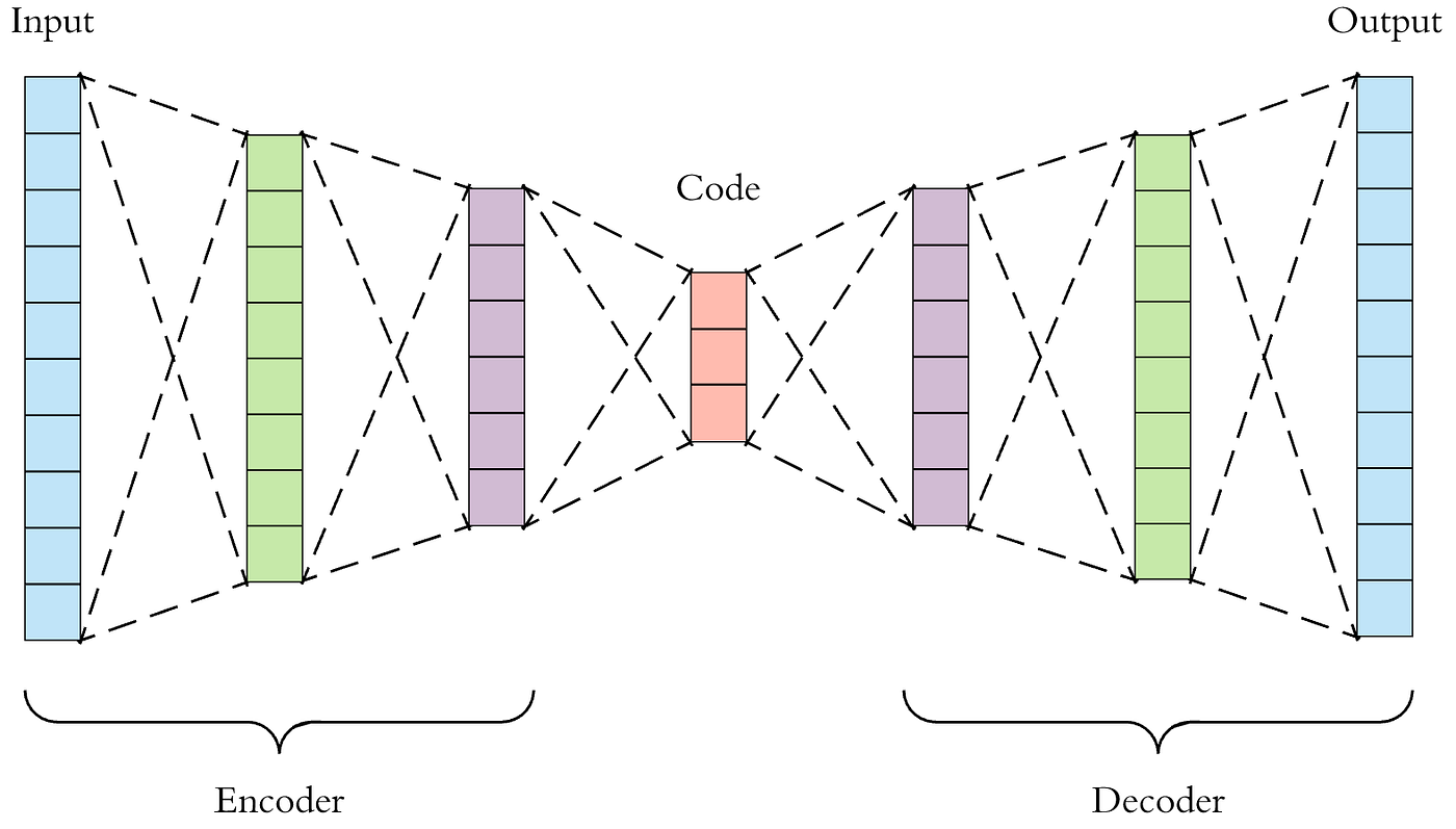
Autoencoder (AE) is an unsupervised learning neural network model whose core goal is to learn a compressed representation of data.

intuitively understands: It’s like “compressing a file and then decompressing it” - compressing a picture into dozens of numbers (encoding), and then restoring the picture from these dozens of numbers (decoding). The bottleneck structure forces the network to cram the most key takeaways of information into a few numbers and automatically learn the essential characteristics of the data.

• architecture: composed of encoder (Encoder) $f_\theta$ and decoder (Decoder) $g_\phi$ Composed of two parts. The encoder compresses the high-dimensional input $\mathbf{x} \in \mathbb{R}^n$ into a low-dimensional latent representation $\mathbf{z} = f_\theta(\mathbf{x}) \in \mathbb{R}^d$ (where $d \ll n$), and the decoder maps $\mathbf{z}$ back to the original space to generate the reconstruction $\hat{\mathbf{x}} = g_\phi(\mathbf{z})$.

• Core idea: Use the “bottleneck” structure (low-dimensional hidden layer) to force the network to learn the most essential features in the data and discard redundant information. It can be compared to a nonlinear PCA.

• loss function: Minimize the reconstruction error, such as mean square error:

\[\mathcal{L} = \|\mathbf{x} - \hat{\mathbf{x}}\|^2 = \|\mathbf{x} - g_\phi(f_\theta(\mathbf{x}))\|^2\]

formula interpretation: $\mathbf{x}$ is the original input, $\hat{\mathbf{x}}$ is the reconstructed output, and the loss is “how distorted the restoration is.” After the training is completed, the hidden vector $\mathbf{z}$ extracted by the encoder $f_\theta$ is the compressed representation of the data ($d \ll n$).

• Main variants:

  • denoising autoencoder (Denoising AE, DAE): Input artificially noisy $\tilde{\mathbf{x}}$, and the training model recovers clean $\mathbf{x}$, forcing the network to learn more robust features.

  • Sparse Autoencoder (Sparse AE): Apply sparse constraints (such as KL divergence penalty) on the hidden layer, so that only a few neurons are activated, resulting in more interpretable features.

  • Contractive AE: Add the Frobenius norm penalty of the encoder Jacobian matrix to the loss to make the hidden layer representation insensitive to small input perturbations.

• Limitations: Ordinary AE does not explicitly match the constraints of sampleable priors; randomly sampled latent vectors may fall in areas rarely covered by training encodings, and decoding quality cannot be guaranteed. This does not mean that the encoding or decoding functions are mathematically discontinuous. Therefore, AE is good at compression and reconstruction, but is not suitable for directly generating new samples. This is exactly the problem that VAE wants to solve.

• application scenarios: nonlinear dimensionality reduction and feature learning, image denoising, anomaly detection (reconstruction error is used as the candidate score, but abnormal samples may also be well reconstructed and need to be verified separately).

Can be tried first	need attention
Data dimensionality reduction, feature learning, image denoising	Need to generate completely new samples (use VAE/Diffusion instead)
Anomaly detection (reconstruction error as anomaly score)	Hidden space interpretability and continuity requirements are high

3.19 Variational autoencoder (VAE)

Core points: VAE specifies priors for latent variables and approximates posteriors with encoders; simultaneously learns reconstructed and sampled generative distributions through variational inference.

Intuition: Ordinary AE gives each input a certain code, while VAE gives a probability distribution of a set of possible codes. Both reconstruction quality and prior constraints are taken into consideration during training, and prior sampling and decoding are performed during generation. It encourages a more organized latent space, but does not guarantee that every sampling point corresponds to a reasonable sample.

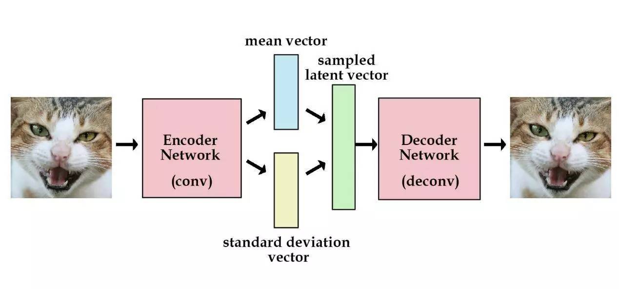
The encoder gives an approximate posterior $q_\phi(\mathbf{z}\mid\mathbf{x})$, the decoder defines the observation distribution $p_\theta(\mathbf{x}\mid\mathbf{z})$, and a commonly used prior is $p(\mathbf{z})=\mathcal{N}(0,I)$. VAE maximizes evidence lower bound (ELBO):

\[\log p_\theta(\mathbf{x}) \geq \mathcal{L}_{\mathrm{ELBO}} = \mathbb{E}_{q_\phi(\mathbf{z}\mid\mathbf{x})}[\log p_\theta(\mathbf{x}\mid\mathbf{z})] - D_{\mathrm{KL}}\big(q_\phi(\mathbf{z}\mid\mathbf{x})\,\|\,p(\mathbf{z})\big)\]

Implementations typically minimize negative ELBO. The first term encourages reconstruction, and the second term constrains the difference between approximate posterior and prior. Under the fixed-variance Gaussian observation model, the negative log-likelihood can be written as the squared reconstruction error with coefficients plus a constant; therefore “reconstructed MSE + KL” is written under specific assumptions and is not a universal accurate goal for all VAEs. Original paper gives variational derivation.

For a diagonal Gaussian posterior, the encoder outputs mean $\boldsymbol{\mu}$ and log variance $\log\boldsymbol{\sigma}^2$, sampled by reparameterization:

\[\mathbf{z}=\boldsymbol{\mu}+\boldsymbol{\sigma}\odot\boldsymbol{\epsilon},\qquad \boldsymbol{\epsilon}\sim\mathcal{N}(0,I)\]

The randomness comes from independent noise, and the gradient can be passed back to the encoder as the mean and standard deviation. Sample directly from the prior when generating, no need to input original samples.

Can be tried first	need attention
Latent variable modeling, data compression, generation and interpolation	Smooth interpolation does not guarantee reasonable semantics, and the sampling quality depends on the model and training.
Provides encoders/decoders for latent space generative models	Simple Gaussian decoders may produce ambiguous results; too strong KL may cause posterior collapse

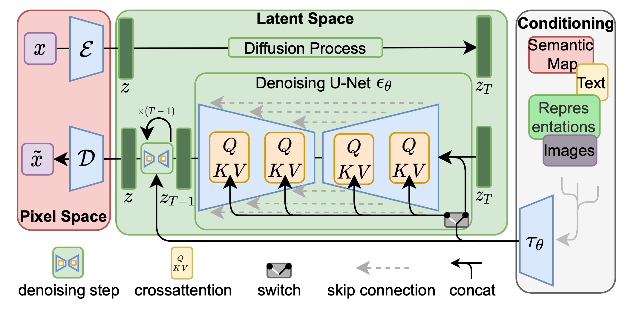
AE, VAE and diffusion models can also be combined: latent space diffusion is first generated on the compressed representation and then the image is restored through the decoder.

3.20 Diffusion Models

Core points: Establish the generation process through learning goals under different noise levels; taking DDPM as an example, train to predict noise, and iteratively update samples when sampling.

Diffusion Models model data distribution by learning the reverse generation process of the noise process. The following takes DDPM as an example; Latent space diffusion performs a similar process on the compressed representation obtained by the encoder to reduce computational costs.

intuitively understands: just like the creative process of a sculptor - not directly carving the finished product, but starting from a piece of marble (pure noise), carefully carving it one by one (denoising each step), and finally presenting a clear work. Each step makes corrections based on the current sample and generation conditions; the results still depend on the model error and sampling settings.

• core idea : Transform the “generation” problem into a “denoising” problem. The model does not directly learn how to generate images from noise in one step, but instead learns how Recover clear images from pure noise step by step .

• forward diffusion process (noising, Fixed): Given a real image \(\mathbf{x}_0\), according to the predefined noise schedule \(\beta_1, \beta_2, \dots, \beta_T\), Gaussian noise is gradually superimposed:

\[q(\mathbf{x}_t | \mathbf{x}_{t-1}) = \mathcal{N}(\mathbf{x}_t; \sqrt{1-\beta_t}\,\mathbf{x}_{t-1}, \beta_t \mathbf{I})\]

With a suitable noise schedule, after enough steps (the original DDPM used $T=1000$), \(\mathbf{x}_T\) becomes approximately pure Gaussian noise \(\mathcal{N}(0, \mathbf{I})\). Using the accumulated parameter \(\bar{\alpha}_t = \prod_{s=1}^t (1-\beta_s)\), you can jump directly from \(\mathbf{x}_0\) to any time step:

\[\mathbf{x}_t = \sqrt{\bar{\alpha}_t}\,\mathbf{x}_0 + \sqrt{1-\bar{\alpha}_t}\,\boldsymbol{\epsilon}\]

• reverse denoising process (generated, Learned): train a noise prediction network \(\boldsymbol{\epsilon}_\theta(\mathbf{x}_t, t)\) (U-Net or Transformer can be used), learn to predict the added noise \(\boldsymbol{\epsilon}\) at each time step $t$. A commonly used simplified noise prediction loss is (it is weighted differently from the full variational objective):

\[\mathcal{L} = \mathbb{E}_{t, \mathbf{x}_0, \boldsymbol{\epsilon}} \left[ \|\boldsymbol{\epsilon} - \boldsymbol{\epsilon}_\theta(\mathbf{x}_t, t)\|^2 \right]\]

Interpretation of the formula: \(\boldsymbol{\epsilon}\) is the actual noise added in the forward process, and \(\boldsymbol{\epsilon}_\theta(\mathbf{x}_t, t)\) is the network’s prediction of this noise at step $t$ - the training goal is to minimize the mean square error of the two. After the training is completed, the generation starts from the pure noise \(\mathbf{x}_T\), repeatedly calling the network to predict and remove the noise, and gradually restores the clear image \(\mathbf{x}_0\).

• condition generation and guidance:

  • Classifier-Free Guidance: Randomly discard conditions during training so that the same network can give conditional and unconditional predictions; combine the two and adjust the guidance strength during inference $w$. Stronger guidance may enhance condition compliance, or it may reduce diversity or produce artifacts. This is a key technology in Vincentian graph models such as Stable Diffusion.

  • Text condition: Convert the text into a vector through an encoder such as CLIP, and inject it into the cross-attention layer of U-Net to achieve “text description → image generation”.

• Comparison between and GAN/VAE: The following table compares the mechanisms of typical implementations, and is not a quality ranking under unified data and budget.

Dimensions	GAN	VAE	diffusion model
learning objectives	Generator versus discriminator	Maximize ELBO	Goals such as denoising and score estimation
Typical sampling path	The noise passes through the generator once forward	The latent variable is passed through the decoder once forward	Iteratively update starting from noise
common difficulties	Confrontation training imbalance and model collapse	Reconstruction and KL trade-off, posterior collapse	Multi-step reasoning cost, guidance and diversity trade-offs
Conditional control	Tags or other conditions can be added	Constructable condition VAE	Conditional networking and bootstrapping available

• Accelerated sampling: DDIM, DPM-Solver, etc. can reduce the number of sampling steps; the number of noise time steps in training is not equal to the number of network calls during inference. Few-step models can also be obtained by distillation, and speed and quality need to be evaluated together.
• application scenario: image generation, editing, audio synthesis and action sequence modeling. Whether it is suitable for real-time tasks requires measuring the latency of the entire system, and cannot be judged by the name “diffusion” alone.

Advanced reading: The following distinguishes three easily confused levels: what network to use (U-Net / Transformer), what variables to generate (image / action), and how to organize the generation process (diffusion / autoregression).

3.20.1 Architecture evolution: Traditional U-Net Diffusion vs DiT (Diffusion Transformer)

diffusion describes the generation and training methods, and U-Net/Transformer describes the network structure. The two are not of the same dimension. Replacing the backbone does not necessarily mean changing the target function; the same Transformer backbone can also use different generation targets.

Dimensions	U-Net backbone	Original DiT
structure	Multi-scale encoder/decoder with skip connection, can add attention	Cut the noisy latent variables into patch tokens and process them with Transformer
structural preference	Locality, multi-scale feature reuse	Token interaction through attention, relying on position and conditional representation
conditional injection	Temporal embedding; text conditional model can add cross-attention	The original paper compares various solutions. The main model uses adaLN-Zero to inject time and category conditions.
Compute concerns	Resolution, number of channels, attention layer configuration	Number of tokens, hidden dimensions and number of layers; global attention has a secondary interaction cost
represent	DDPM, Stable Diffusion 1.x/2.x	DiT(Peebles & Xie, ICCV 2023)

DiT original paper observed within the scope of their ImageNet experiments that increasing model computation was associated with lower FID. This supports the scalability potential of this structure, but does not constitute a law of “outperform U-Net at any scale and on any data”. U-Net with attention can also model global relationships, and it cannot be simply described as having only local receptive fields.

The difference between DiT and Flow Matching: DiT is an architectural choice; Flow Matching generates samples by learning the velocity field on a continuous path. Stable Diffusion 3 uses Rectified Flow with a multi-modal Transformer and cannot be directly equated to “original DiT + DDPM noise loss”. The relevant mechanism can be found in SD3 paper .

3.20.2 Diffusion Policy: Application of diffusion model in robot decision-making

Diffusion Policy (Chi et al., 2023) is a imitation learning method: learning an observation-conditioned action distribution from demonstration data. It is not a reinforcement learning algorithm per se trained with rewards, nor does it necessarily include language input.

Let the observation condition be \(\mathbf{o}_t\), the prediction length be $H$, and the action clip be \(\mathbf{A}_t=(\mathbf{a}_t,\ldots,\mathbf{a}_{t+H-1})\). Add noise to the demonstration actions during training and learn conditional noise prediction:

\[\mathcal{L}_{\mathrm{policy}} = \mathbb{E}_{\mathbf{A}_t,\mathbf{o}_t,k,\boldsymbol{\epsilon}}\left[\left\|\boldsymbol{\epsilon}-\boldsymbol{\epsilon}_\theta(\mathbf{A}_t^{(k)},k,\mathbf{o}_t)\right\|^2\right]\]

Here $t$ is the environment time and $k$ is the diffusion time step. The two cannot be mixed. During inference, segments are generated from action noise, only part of them are executed, and then re-planned based on new observations, that is, rolling time domain control.

• Multimodal action distribution: There may be two reasonable paths, left and right, around obstacles. Deterministic MSE regression might output a mean path; conditional diffusion can express multiple modes, but other probabilistic strategies can also model multimodal distributions.
• action clip: Joint prediction of multiple time steps helps timing consistency; it still needs to face model errors, environmental changes and closed-loop distribution shifts, and error accumulation cannot be guaranteed to be eliminated.
• Architecture and Cost: The original work has studied two types of implementations: convolution and Transformer, and Transformer was not introduced later. Control frequency is also affected by the number of denoising steps, visual encoding, and hardware.

Related work needs to be distinguished by goal: RDT-1B uses diffusion action modeling; π₀ uses Flow Matching and is combined with a pretrained visual language model. Both can iteratively generate continuous actions, but the training objectives cannot be confused with the same DDPM denoising loss. When comparing performance, it is also necessary to align demonstration data, robot morphology, and mission protocols.

3.20.3 Diffusion architecture vs autoregressive architecture: Comparison of two generative paradigms

Autoregressive (AR) decomposes the joint distribution according to conditional probability; diffusion generates samples through a multi-step reverse process. Both can use Transformers, and both can express multimodal distributions.

Dimensions	autoregressive	Diffusion (taking common continuous diffusion as an example)
probabilistic organization	\(p(x)=\prod_i p(x_i\mid x_{<i})\)	Step by step update the entire sample starting from the noise
training and inference	Teacher forcing training of standard Transformer can be parallelized; typical samples are generated in steps	Training can sample noise time steps; different time steps are executed sequentially during sampling, and positions within steps can be parallelized.
Output length	Common terminators generate variable-length sequences	The shape or length is often preset, and length conditions and blocking mechanisms can also be added.
Source of error	Model conditional distribution error, and training/inference context differences	Denoising prediction error, sampling discretization error and conditional distribution shift
Likely	If each conditional distribution can be evaluated, the sequence likelihood can be calculated	DDPM often uses variational bounds; other forms also have different likelihood estimation methods
data type	Commonly seen in discrete tokens, continuous conditional distributions can also be output.	Common in continuous signals, but also in discrete diffusion
cost factor	Output length, cache, network cost per step and decoding method	Number of denoising steps, output size, network cost and sampler

Therefore, “Autoregression is only suitable for discrete data”, “Diffusion has no error accumulation” and “Diffusion must be faster than autoregression” are not universal conclusions. Selection should be based on comparing quality, coverage, controllability, and end-to-end latency with similar data and budget.

For text diffusion, please refer to LLaDA; for hybrid modeling, please refer to Transfusion, which combines text autoregressive objectives and image diffusion objectives in one model. These works demonstrate that different generative approaches can be combined, rather than necessarily substituted for each other.

4. Summary

4.1 How to choose the first model

First establish candidates based on data format and task constraints, and then compare using the same division and indicators. The following is a starting plan, not a final ranking.

Problems and Constraints	Starting plan	What to check next
Tabular regression or classification, need to be easy to diagnose	regularization linear/logistic regression, versus random forest or gradient boosting tree	Are nonlinear interactions important and are the returns of complex models stable?
High-dimensional sparse text classification	TF-IDF + Logistic Regression, Linear SVM or Naive Bayes	Whether the error comes from insufficient semantics and context, and whether pre-training representation is required
Image tasks, the amount of annotation is limited	Feature/fine-tuning of pretrained CNN or visual Transformer	Data augmentation, domain differences, input resolution and latency
Time series or streaming signal	Seasonal/lagged baselines, compared to tree models, RNNs or other sequence networks	Is the time division reasonable? Is there any future information leakage?
Structural exploration and visualization	Comparison of PCA and K-Means after normalization; t-SNE auxiliary observation	Is the distance metric reasonable and does the structure change with settings?
Open language or multimodal generation	Pre-trained generative models suitable for the task	Task accuracy, condition compliance, computational cost and output reliability
Robot Demonstration Learning	Simple behavioral clone baselines against action clips or generative strategies	Closed-loop success rate, recovery capability, control frequency and data coverage

4.2 Reading and Practice Sequence

1. First master the experimental method: Starting from linear/logistic regression, understand loss, regularization, data division and evaluation indicators.
2. Compare the structural hypothesis again: Use the same task to compare trees, distance methods and neural networks to observe how they utilize features and samples.
3. finally studies pre-training and generation: understands representation transfer, probabilistic modeling and conditional generation, and then goes deeper into Transformer, VAE, diffusion and policy learning.

The training details of deep networks can be extended to read “Review of deep learning” ; when it comes to reward-driven sequence decision-making, you can read “Review of reinforcement learning” .

To understand a method, you must at least be able to explain it Learning signals, structural assumptions, optimization goals and failure conditions . Only with a credible verification design can model comparison be meaningful; only with error analysis can there be a clear direction by increasing data and complexity.

References

1. Hastie, T., Tibshirani, R., & Friedman, J. (2009). The Elements of Statistical Learning: Data Mining, Inference, and Prediction (2nd ed.). Springer.
2. Bishop, C. M. (2006). Pattern Recognition and Machine Learning. Springer.
3. Goodfellow, I., Bengio, Y., & Courville, A. (2016). Deep Learning. MIT Press. https://www.deeplearningbook.org/
4. Sutton, R. S., & Barto, A. G. (2018). Reinforcement Learning: An Introduction (2nd ed.). MIT Press.
5. Tibshirani, R. (1996). Regression Shrinkage and Selection via the Lasso. Journal of the Royal Statistical Society, Series B, 58(1), 267–288.
6. Quinlan, J. R. (1986). Induction of Decision Trees. Machine Learning, 1(1), 81–106. (ID3)
7. Quinlan, J. R. (1993). C4.5: Programs for Machine Learning. Morgan Kaufmann.
8. Breiman, L., Friedman, J., Olshen, R., & Stone, C. (1984). Classification and Regression Trees. Wadsworth. (CART)
9. Breiman, L. (2001). Random Forests. Machine Learning, 45(1), 5–32.
10. Friedman, J. H. (2001). Greedy Function Approximation: A Gradient Boosting Machine. The Annals of Statistics, 29(5), 1189–1232. (GBDT)
11. Chen, T., & Guestrin, C. (2016). XGBoost: A Scalable Tree Boosting System. KDD 2016. arXiv:1603.02754
12. Ke, G., et al. (2017). LightGBM: A Highly Efficient Gradient Boosting Decision Tree. NeurIPS 2017.
13. Cover, T., & Hart, P. (1967). Nearest Neighbor Pattern Classification. IEEE Transactions on Information Theory, 13(1), 21–27. (KNN)
14. Rabiner, L. R. (1989). A Tutorial on Hidden Markov Models and Selected Applications in Speech Recognition. Proceedings of the IEEE, 77(2), 257–286.
15. Cortes, C., & Vapnik, V. (1995). Support-Vector Networks. Machine Learning, 20(3), 273–297.
16. MacQueen, J. (1967). Some Methods for Classification and Analysis of Multivariate Observations. Proc. 5th Berkeley Symp. on Math. Statist. and Prob. (K-Means)
17. Pearson, K. (1901). On Lines and Planes of Closest Fit to Systems of Points in Space. Philosophical Magazine, 2(11), 559–572. (PCA)
18. van der Maaten, L., & Hinton, G. (2008). Visualizing Data using t-SNE. Journal of Machine Learning Research, 9, 2579–2605.
19. Rumelhart, D. E., Hinton, G. E., & Williams, R. J. (1986). Learning Representations by Back-Propagating Errors. Nature, 323(6088), 533–536.
20. Hornik, K., Stinchcombe, M., & White, H. (1989). Multilayer Feedforward Networks are Universal Approximators. Neural Networks, 2(5), 359–366.
21. Kingma, D. P., & Ba, J. (2015). Adam: A Method for Stochastic Optimization. ICLR 2015. arXiv:1412.6980
22. LeCun, Y., Bottou, L., Bengio, Y., & Haffner, P. (1998). Gradient-Based Learning Applied to Document Recognition. Proceedings of the IEEE, 86(11), 2278–2324. (LeNet-5)
23. Krizhevsky, A., Sutskever, I., & Hinton, G. E. (2012). ImageNet Classification with Deep Convolutional Neural Networks. NeurIPS 2012. (AlexNet)
24. Simonyan, K., & Zisserman, A. (2015). Very Deep Convolutional Networks for Large-Scale Image Recognition. ICLR 2015. arXiv:1409.1556 (VGG)
25. He, K., Zhang, X., Ren, S., & Sun, J. (2016). Deep Residual Learning for Image Recognition. CVPR 2016. arXiv:1512.03385 (ResNet)
26. Hochreiter, S., & Schmidhuber, J. (1997). Long Short-Term Memory. Neural Computation, 9(8), 1735–1780.
27. Cho, K., et al. (2014). Learning Phrase Representations using RNN Encoder-Decoder for Statistical Machine Translation. EMNLP 2014. arXiv:1406.1078 (GRU)
28. Vaswani, A., et al. (2017). Attention Is All You Need. NeurIPS 2017. arXiv:1706.03762
29. Su, J., et al. (2021). RoFormer: Enhanced Transformer with Rotary Position Embedding. arXiv:2104.09864 (RoPE)
30. Press, O., Smith, N. A., & Lewis, M. (2022). Train Short, Test Long: Attention with Linear Biases Enables Input Length Extrapolation. ICLR 2022. (ALiBi)
31. Devlin, J., Chang, M. W., Lee, K., & Toutanova, K. (2019). BERT: Pre-training of Deep Bidirectional Transformers for Language Understanding. NAACL 2019. arXiv:1810.04805
32. Liu, Y., et al. (2019). RoBERTa: A Robustly Optimized BERT Pretraining Approach. arXiv:1907.11692
33. Lan, Z., et al. (2020). ALBERT: A Lite BERT for Self-supervised Learning of Language Representations. ICLR 2020.
34. He, P., et al. (2021). DeBERTa: Decoding-Enhanced BERT with Disentangled Attention. ICLR 2021.
35. Radford, A., et al. (2018). Improving Language Understanding by Generative Pre-Training. OpenAI Tech Report. (GPT-1)
36. Radford, A., et al. (2019). Language Models are Unsupervised Multitask Learners. OpenAI Tech Report. (GPT-2)
37. Brown, T. B., et al. (2020). Language Models are Few-Shot Learners. NeurIPS 2020. arXiv:2005.14165 (GPT-3)
38. OpenAI. (2023). GPT-4 Technical Report. arXiv:2303.08774
39. Kaplan, J., et al. (2020). Scaling Laws for Neural Language Models. arXiv:2001.08361
40. Wei, J., et al. (2022). Emergent Abilities of Large Language Models. TMLR 2022. arXiv:2206.07682
41. Wei, J., et al. (2022). Chain-of-Thought Prompting Elicits Reasoning in Large Language Models. NeurIPS 2022. arXiv:2201.11903
42. Ouyang, L., et al. (2022). Training Language Models to Follow Instructions with Human Feedback. NeurIPS 2022. arXiv:2203.02155 (InstructGPT / RLHF)
43. Rafailov, R., et al. (2023). Direct Preference Optimization: Your Language Model is Secretly a Reward Model. NeurIPS 2023. arXiv:2305.18290 (DPO)
44. Goodfellow, I., et al. (2014). Generative Adversarial Nets. NeurIPS 2014. arXiv:1406.2661
45. Arjovsky, M., Chintala, S., & Bottou, L. (2017). Wasserstein GAN. ICML 2017. arXiv:1701.07875
46. Karras, T., Laine, S., & Aila, T. (2019). A Style-Based Generator Architecture for Generative Adversarial Networks. CVPR 2019. (StyleGAN)
47. Zhu, J. Y., et al. (2017). Unpaired Image-to-Image Translation using Cycle-Consistent Adversarial Networks. ICCV 2017. (CycleGAN)
48. Vincent, P., et al. (2008). Extracting and Composing Robust Features with Denoising Autoencoders. ICML 2008.
49. Kingma, D. P., & Welling, M. (2014). Auto-Encoding Variational Bayes. ICLR 2014. arXiv:1312.6114 (VAE)
50. Ho, J., Jain, A., & Abbeel, P. (2020). Denoising Diffusion Probabilistic Models. NeurIPS 2020. arXiv:2006.11239 (DDPM)
51. Song, J., Meng, C., & Ermon, S. (2021). Denoising Diffusion Implicit Models. ICLR 2021. arXiv:2010.02502 (DDIM)
52. Lu, C., et al. (2022). DPM-Solver: A Fast ODE Solver for Diffusion Probabilistic Model Sampling. NeurIPS 2022.
53. Ho, J., & Salimans, T. (2022). Classifier-Free Diffusion Guidance. arXiv:2207.12598
54. Rombach, R., et al. (2022). High-Resolution Image Synthesis with Latent Diffusion Models. CVPR 2022. arXiv:2112.10752 (Stable Diffusion)
55. Ramesh, A., et al. (2022). Hierarchical Text-Conditional Image Generation with CLIP Latents. arXiv:2204.06125 (DALL-E 2)
56. Peebles, W., & Xie, S. (2023). Scalable Diffusion Models with Transformers. ICCV 2023. arXiv:2212.09748 (DiT)
57. Brooks, T., et al. (2024). Video Generation Models as World Simulators. OpenAI Tech Report. (Sora)
58. Chen, J., et al. (2024). PixArt-α: Fast Training of Diffusion Transformer for Photorealistic Text-to-Image Synthesis. ICLR 2024.
59. Esser, P., et al. (2024). Scaling Rectified Flow Transformers for High-Resolution Image Synthesis. ICML 2024. arXiv:2403.03206 (Stable Diffusion 3)
60. Chi, C., et al. (2023). Diffusion Policy: Visuomotor Policy Learning via Action Diffusion. RSS 2023. arXiv:2303.04137
61. Ze, Y., et al. (2024). 3D Diffusion Policy. RSS 2024.
62. Liu, S., et al. (2024). RDT-1B: A Diffusion Foundation Model for Bimanual Manipulation. arXiv:2410.07864
63. Black, K., et al. (2024). π₀: A Vision-Language-Action Flow Model for General Robot Control. Physical Intelligence. arXiv:2410.24164
64. Octo Model Team. (2024). Octo: An Open-Source Generalist Robot Policy. RSS 2024.
65. Kim, M. J., et al. (2024). OpenVLA: An Open-Source Vision-Language-Action Model. arXiv:2406.09246
66. Tian, K., et al. (2024). Visual Autoregressive Modeling: Scalable Image Generation via Next-Scale Prediction. NeurIPS 2024. (VAR)
67. Zhou, C., et al. (2024). Transfusion: Predict the Next Token and Diffuse Images with One Multi-Modal Model. arXiv:2408.11039
68. Nie, S., et al. (2025). Large Language Diffusion Models. arXiv:2502.09992 (LLaDA)
69. Deng, J., et al. (2009). ImageNet: A Large-Scale Hierarchical Image Database. CVPR 2009.
70. Lin, T. Y., et al. (2014). Microsoft COCO: Common Objects in Context. ECCV 2014.
71. Wang, A., et al. (2019). GLUE: A Multi-Task Benchmark and Analysis Platform for Natural Language Understanding. ICLR 2019.
72. Pedregosa, F., et al. (2011). Scikit-learn: Machine Learning in Python. JMLR, 12, 2825–2830.
73. Abadi, M., et al. (2016). TensorFlow: Large-Scale Machine Learning on Heterogeneous Distributed Systems. arXiv:1603.04467
74. Paszke, A., et al. (2019). PyTorch: An Imperative Style, High-Performance Deep Learning Library. NeurIPS 2019.
75. Wolf, T., et al. (2020). Transformers: State-of-the-Art Natural Language Processing. EMNLP 2020 (System Demos). (HuggingFace)
76. Jumper, J., et al. (2021). Highly Accurate Protein Structure Prediction with AlphaFold. Nature, 596, 583–589.
77. Silver, D., et al. (2016). Mastering the Game of Go with Deep Neural Networks and Tree Search. Nature, 529, 484–489. (AlphaGo)
78. Mnih, V., et al. (2015). Human-Level Control through Deep Reinforcement Learning. Nature, 518, 529–533. (DQN)
79. Schulman, J., et al. (2017). Proximal Policy Optimization Algorithms. arXiv:1707.06347 (PPO)

80. Haarnoja, T., et al. (2018). Soft Actor-Critic: Off-Policy Maximum Entropy Deep Reinforcement Learning with a Stochastic Actor. ICML 2018. (SAC)

81. Scikit-learn developers. Common pitfalls and recommended practices; Cross-validation; Metrics and scoring.
82. Schaeffer, R., Miranda, B., & Koyejo, S. (2023). Are Emergent Abilities of Large Language Models a Mirage? NeurIPS 2023. arXiv:2304.15004

Reading Tips: The pictures are provided to assist understanding; please refer to the corresponding original paper for specific algorithm definitions, training settings and experimental conclusions.